Skip to the Main Content

Note:These pages make extensive use of the latest XHTML and CSS Standards. They ought to look great in any standards-compliant modern browser. Unfortunately, they will probably look horrible in older browsers, like Netscape 4.x and IE 4.x. Moreover, many posts use MathML, which is, currently only supported in Mozilla. My best suggestion (and you will thank me when surfing an ever-increasing number of sites on the web which have been crafted to use the new standards) is to upgrade to the latest version of your browser. If that's not possible, consider moving to the Standards-compliant and open-source Mozilla browser.

August 28, 2017

Schröder Paths and Reverse Bessel Polynomials

Posted by Simon Willerton

I want to show you a combinatorial interpretation of the reverse Bessel polynomials which I learnt from Alan Sokal. The sequence of reverse Bessel polynomials begins as follows.

θ 0(R) =1 θ 1(R) =R+1 θ 2(R) =R 2+3R+3 θ 3(R) =R 3+6R 2+15R+15 \begin{aligned} \theta_0(R)&=1\\ \theta_1(R)&=R+1\\ \theta_2(R)&=R^2+3R+3\\ \theta_3(R)&= R^3 +6R^2+15R+15 \end{aligned}

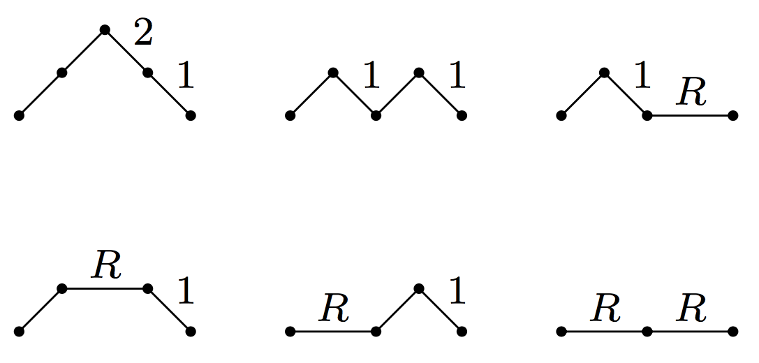
To give you a flavour of the combinatorial interpretation we will prove, you can see that the second reverse Bessel polynomial can be read off the following set of ‘weighted Schröder paths’: multiply the weights together on each path and add up the resulting monomials.

Schroeder paths

In this post I’ll explain how to prove the general result, using a certain result about weighted Dyck paths that I’ll also prove. At the end I’ll leave some further questions for the budding enumerative combinatorialists amongst you.

These reverse Bessel polynomials have their origins in the theory of Bessel functions, but which I’ve encountered in the theory of magnitude, and they are key to a formula I give for the magnitude of an odd dimensional ball which I have just posted on the arxiv.

In that paper I use the combinatorial expression for these Bessel polynomials to prove facts about the magnitude.

Here, to simplify things slightly, I have used the standard reverse Bessel polynomials whereas in my paper I use a minor variant (see below).

I should add that a very similar expression can be given for the ordinary, unreversed Bessel polynomials; you just need a minor modification to the way the weights on the Schröder paths are defined. I will leave that as an exercise.

The reverse Bessel polynomials

The reverse Bessel polynomials have many properties. In particular they satisfy the recursion relation θ i+1(R)=R 2θ i1(R)+(2i+1)θ i(R) \theta_{i+1}(R)=R^2\theta_{i-1}(R) + (2i+1)\theta_{i}(R) and θ i(R)\theta_i(R) satisfies the differential equation Rθ i (R)2(R+i)θ i (R)+2iθ i(R)=0. R\theta_i^{\prime\prime}(R)-2(R+i)\theta_i^\prime(R)+2i\theta_i(R)=0. There’s an explicit formula: θ i(R)= t=0 i(i+t)!(it)!t!2 tR it. \theta_i(R) = \sum_{t=0}^i \frac{(i+t)!}{(i-t)!\, t!\, 2^t}R^{i-t}.

I’m interested in them because they appear in my formula for the magnitude of odd dimensional balls. To be more precise, in my formula I use the associated Sheffer polynomials, (χ i(R)) i=0 (\chi_i(R))_{i=0}^\infty; they are related by χ i(R)=Rθ i1(R)\chi_i(R)=R\theta_{i-1}(R), so the coefficients are the same, but just moved around a bit. These polynomials have a similar but slightly more complicated combinatorial interpretation.

In my paper I prove that the magnitude of the (2p+1)(2p+1)-dimensional ball of radius RR has the following expression:

|B R 2p+1|=det[χ i+j+2(R)] i,j=0 p(2p+1)!Rdet[χ i+j(R)] i,j=0 p \left|B^{2p+1}_R \right|= \frac{\det[\chi_{i+j+2}(R)]_{i,j=0}^p}{(2p+1)!\, R\,\det[\chi_{i+j}(R)]_{i,j=0}^p}

As the each polynomial χ i(R)\chi_i(R) has a path counting interpretation, one can use the rather beautiful Lindström-Gessel-Viennot Lemma to give a path counting interpretation to the determinants in the above formula and find some explicit expression. I will probably blog about this another time. (Fellow host Qiaochu has also blogged about the LGV Lemma.)

Weighted Dyck paths

Before getting on to Bessel polynomials and weighted Schröder paths, we need to look at counting weighted Dyck paths, which are simpler and more classical.

A Dyck path is a path in the lattice 2\mathbb{Z}^2 which starts at (0,0)(0,0), stays in the upper half plane, ends back on the xx-axis at (2i,0)(2{i},0) and has steps going either diagonally right and up or right and down. The integer 2i2{i} is called the length of the path. Let D iD_{i} be the set of length 2i2{i} Dyck paths.

For each Dyck path σ\sigma, we will weight each edge going right and down, from (x,y)(x,y) to (x+1,y1)(x+1,y-1) by yy then we will take w(σ)w(\sigma), the weight of σ\sigma, to be the product of all the weights on its steps. Here are all five weighted Dyck paths of length six.

Dyck paths

Famously, the number of Dyck paths of length 2i2{i} is given by the i{i}th Catalan number; here, however, we are interested in the number of paths weighted by the weighting(!). If we sum over the weights of each of the above diagrams we get 6+4+2+2+1=156+4+2+2+1=15. Note that this is 5×3×15\times 3 \times 1. This is a pattern that holds in general.

Theorem A. (Françon and Viennot) The weighted count of length 2i2{i} Dyck paths is equal to the double factorial of 2i12{i} -1: σD iw(σ) =(2i1)(2i3)(2i5)31 (2i1)!!. \begin{aligned} \sum_{\sigma\in D_{i}} w(\sigma)&= (2{i} -1)\cdot (2{i} -3)\cdot (2{i}-5)\cdot \cdots\cdot 3\cdot 1 \\ &\eqqcolon (2{i} -1)!!. \end{aligned}

The following is a nice combinatorial proof of this theorem that I found in a survey paper by Callan. (I was only previously aware of a high-tech proof involving continued fractions and a theorem of Gauss.)

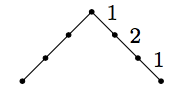
The first thing to note is that the weight of a Dyck path is actually counting something. It is counting the ways of labelling each of the down steps in the diagram by a positive integer less than the height (i.e.~the weight) of that step. We call such a labelling a height labelling. Note that we have no choice of weighting but we often have choice of height labelling. Here’s a height labelled Dyck path.

height labelled Dyck path

So the weighted count of Dyck paths of length 2i2{i} is precisely the number of height labelled Dyck paths of length 2i2{i}. σD iw(σ)=#{height labelled paths of length 2i} \sum_{\sigma\in D_{i}} w(\sigma) = \#\{\text{height labelled paths of length }\,\,2{i}\}

We are going to consider marked Dyck paths, which just means we single out a specific vertex. A path of length 2i2{i} has 2i+12{i} + 1 vertices. Thus

#{height labelled, MARKED paths of length 2i} =(2i+1)×#{height labelled paths of length 2i}. \begin{aligned} \#\{\text{height labelled,}\,\, &\text{ MARKED paths of length }\,\,2{i}\}\\ &=(2{i}+1)\times\#\{\text{height labelled paths of length }\,\,2{i}\}. \end{aligned}

Hence the theorem will follow by induction if we find a bijection

{height labelled, paths of length 2i} {height labelled, MARKED paths of length 2i2}. \begin{aligned} \{\text{height labelled,}\,\,&\text{ paths of length }\,\,2{i} \}\\ &\cong \{\text{height labelled, MARKED paths of length }\,\,2{i}-2 \}. \end{aligned}

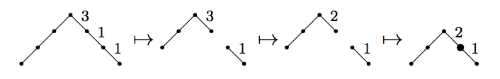
Such a bijection can be constructed in the following way. Given a height labelled Dyck path, remove the left-hand step and the first step that has a label of one on it. On each down step between these two deleted steps decrease the label by one. Now join the two separated parts of the path together and mark the vertex at which they are joined. Here is an example of the process.

dyck bijection

Working backwards it is easy to describe the inverse map. And so the theorem is proved.

Schröder paths and reverse Bessel polynomials

In order to give a path theoretic interpretation of reverse Bessel polynomials we will need to use Schröder paths. These are like Dyck paths except we allow a certain kind of flat step.

A Schröder path is a path in the lattice 2\mathbb{Z}^2 which starts at (0,0)(0,0), stays in the upper half plane, ends back on the xx-axis at (2i,0)(2{i},0) and has steps going either diagonally right and up, diagonally right and down, or horizontally two units to the right. The integer 2i2{i} is called the length of the path. Let S iS_{i} be the set of all length 2i2{i} Schröder paths.

For each Schröder path σ\sigma, we will weight each edge going right and down, from (x,y)(x,y) to (x+1,y1)(x+1,y-1) by yy and we will weight each flat edge by the indeterminate RR. Then we will take w(σ)w(\sigma), the weight of σ\sigma, to be the product of all the weights on its steps.

Here is the picture of all six length four weighted Schröder paths again.

Schroeder paths

You were asked at the top of this post to check that the sum of the weights equals the second reverse Bessel polynomial. Of course that result generalizes!

The following theorem was shown to me by Alan Sokal, he proved it using continued fractions methods, but these essentially amount to the combinatorial proof I’m about to give.

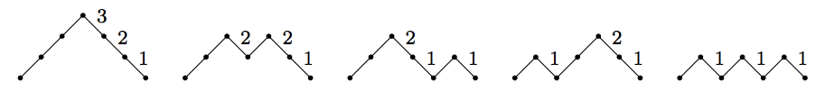
Theorem B. The weighted count of length 2i2{i} Schröder paths is equal to the i{i}th reverse Bessel polynomial: σS iw(σ)=θ i(R). \sum_{\sigma\in S_{i}} w(\sigma)= \theta_{i}(R).

The idea is to observe that you can remove the flat steps from a weighted Schröder path to obtain a weighted Dyck path. If a Schröder path has length 2i2{i} and tt upward steps then it has tt downward steps and it{i}-t flat steps, so it has a total of i+t{i}+t steps. This means that there are (i+tit)\binom{{i}+t}{{i}-t} length 2i2{i} Schröder paths with the same underlying length 2t2t Dyck path (we just choose were to insert the flat steps). Let’s write S i tS^t_{i} for the set of Schröder paths of length 2i2{i} with tt upward steps. σS iw(σ) = t=0 i σS i tw(σ)= t=0 i(i+tit) σD tw(σ)R it = t=0 i(i+tit)(2t1)!!R it = t=0 i(i+t)!(it)!(2t)!(2t)!2 tt!R it =θ i(R), \begin{aligned} \sum_{\sigma\in S_{i}} w(\sigma) &= \sum_{t=0}^{i} \sum_{\sigma\in S^t_{i}} w(\sigma) = \sum_{t=0}^{i} \binom{{i}+t}{{i}-t}\sum_{\sigma'\in D_t} w(\sigma')R^{{i}-t}\\ &= \sum_{t=0}^{i} \binom{{i}+t}{{i}-t}(2t-1)!!\,R^{{i}-t}\\ &= \sum_{t=0}^{i} \frac{({i}+t)!}{({i}-t)!\,(2t)!}\frac{(2t)!}{2^t t!}R^{{i}-t}\\ &= \theta_{i}(R), \end{aligned} where the last equality comes from the formula for θ i(R)\theta_{i}(R) given at the beginning of the post.

Thus we have the required combinatorial interpretation of the reverse Bessel polynomials.

Further questions

The first question that springs to mind for me is if it is possible to give a bijective proof of Theorem B, similar in style, perhaps (or perhaps not), to the proof given of Theorem A, basically using the recursion relation θ i+1(R)=R 2θ i1(R)+(2i+1)θ i(R) \theta_{i+1}(R)=R^2\theta_{i-1}(R) + (2i+1)\theta_{i}(R) rather than the explicit formular for them.

The second question would be whether the differential equation Rθ i (R)2(R+i)θ i (R)+2iθ i(R)=0. R\theta_i^{\prime\prime}(R)-2(R+i)\theta_i^\prime(R)+2i\theta_i(R)=0. has some sort of combinatorial interpretation in terms of paths.

I’m interested to hear if anyone has any thoughts.

Posted at August 28, 2017 1:09 PM UTC

TrackBack URL for this Entry:   https://golem.ph.utexas.edu/cgi-bin/MT-3.0/dxy-tb.fcgi/2980

12 Comments & 0 Trackbacks

Re: Schröder Paths and Reverse Bessel Polynomials

Interesting post! One thing that comes to mind: have you tried considering the reverse Bessel polynomials in terms of involutions, or equivalently in terms of rooted chord diagrams? There is a simple bijection between height labelled Dyck paths and fixed point free involutions, which I think is easiest to visualize using the representation of involutions by diagrams: scanning a labelled Dyck path from left to right, every NE step introduces a rising arc, while every SE(ii) step introduces a falling arc that closes the iith unattached arc. For example, the height labelled Dyck path NE NE NE SE(1) SE(2) SE(1) from your example corresponds to the rooted chord diagram

rooted chord diagram

and to the fixed point free involution (1 4)(2 6)(3 5).

This interpretation extends to weighted Schröder paths by allowing rooted chord diagrams with unattached marked points, hence fixed points of the corresponding involution. For example, under this interpretation the weighted Schröder path NE EE SE(1) corresponds to the involution (1 3)(2), while the path EE NE SE(1) corresponds to the involution (1) (2 3).

I don’t quite see how to interpret the recursion relation for θ i(R)\theta_i(R) in terms of involutions/chord diagrams. However, consider the formal power series which gathers together all of the reverse Bessel polynomials: θ(z,x)= iθ i(x)z i \theta(z,x) = \sum_i \theta_i(x) z^i Reinterpreting weighted Schröder paths as involutions, Theorem B implies that θ(z,x)\theta(z,x) can be seen as the bivariate generating function counting involutions by total number of cycles (zz) and number of 1-cycles/fixed points (xx). I wonder whether it might potentially be useful to consider the reparameterization θ(z,x)=κ(zx,x) \theta(z,x) = \kappa(z x,x) where κ(z,x)\kappa(z,x) is the bivariate generating function counting involutions by number of 2-cycles (zz) and 1-cycles (xx) (or equivalently, rooted chord diagrams by number of chords and number of marked points)? In particular, κ(z,x)\kappa(z,x) satisfies the functional-differential equation κ(z,x)=1+xκ(z,x)+zκ(z,x)x \kappa(z,x) = 1 + x\kappa(z,x) + z\frac{\partial \kappa(z,x)}{\partial x} which has the following simple interpretation: starting from the empty rooted chord diagram (1), we can build a larger diagram either by adding an unattached point at the end of a smaller diagram (xκ(z,x)x\kappa(z,x)), or by picking an unattached point of the smaller diagram and closing it with a chord (zκ(z,x)xz\frac{\partial \kappa(z,x)}{\partial x}).

Posted by: Noam Zeilberger on August 30, 2017 1:16 PM | Permalink | Reply to this

Re: Schröder Paths and Reverse Bessel Polynomials

Ah, interesting. As you know, because you seem to have written the nLab page on chord diagrams, I have had quite an interest in chord diagrams in the past in relation to Vassiliev knot invariants.

Anyway, what you’re saying then, is if we let I iI_i be the set of involutions consisting of ii cycles then the iith reverse Bessel polynomial has the following interpretation:

θ i(R) = σI iR #fix(σ) = k=0 i#{involutions withicycles andkfixed points}R k \begin{aligned} \theta_i(R) &= \sum_{\sigma\in I_i} R^{\# fix(\sigma)}\\ &=\sum_{k=0}^{i}\#\{\text{involutions with}\,\,i\,\,\text{cycles and}\,\,k\,\, \text{fixed points}\}\,R^k \end{aligned}

This seems a little odd in some sense that we’re not saying what set the involution is acting on. Indeed, I can’t think of a good way of saying it without it sounding artificial.

I had a play, but I couldn’t make the recursion work.

Posted by: Simon Willerton on August 30, 2017 11:28 PM | Permalink | Reply to this

Re: Schröder Paths and Reverse Bessel Polynomials

Well, to be formal we should probably take I iI_i to be the set of isomorphism classes of linearly ordered sets (X,)(X,\le) equipped with an involution σ:XX\sigma : X \to X with ii cycles, or equivalently, isomorphism classes of rooted chord diagrams with some number kk of marked points and iki-k chords.

I’m not sure whether the reparameterization and the differential equation I suggested above are actually useful (also, there was a small bug: that should be θ(z,x)=κ(z,zx)\theta(z,x) = \kappa(z,z x)), but I did find an abstract for a paper by Serge Dulucq and Luc Favreau on A combinatorial model for Bessel polynomials “based upon weighted involutions” that looks encouraging. Sadly, that paper does not seem to be available online, but there is another short followup paper by Dulucq that at least gives a hint of what they did. There, Dulucq defines a q-analogue of the (ordinary, rather than reverse) Bessel polynomials by y n(x;q)= k=0 n αI n,kq s(α)x k y_n(x;q) = \sum_{k=0}^n \sum_{\alpha \in I_{n,k}} q^{s(\alpha)} x^k where I n,kI_{n,k} is the set of involutions with nn cycles and kk 2-cycles, and s()s(-) is a certain weighting function on involutions. He states q-analogues of the explicit formula and the recurrence relation for the y ny_n as theorems, but sadly there are no proofs.

Posted by: Noam Zeilberger on August 31, 2017 4:01 AM | Permalink | Reply to this

Re: Schröder Paths and Reverse Bessel Polynomials

Oh, the proofs are in Chapter 4 of Favreau’s thesis! It’s in French, but with lots of illustrations…in particular, Figure 4.3 on p.78 gives a graphical bijection (using rooted chord diagrams!) to account for the recurrence relation defining the Bessel polynomials. The text refers to the ordinary Bessel polynomials, but the same exact bijection also works for the reverse Bessel polynomials – here is a sketch of Favreau’s argument, translated in reverse:

Consider an involution σ\sigma with n+1n+1 cycles and kk fixed points on a linearly ordered set, represented as a rooted chord diagram. We examine the rightmost point xx of the diagram (i.e., the greatest element of the underlying set). There are two possiblities:

  • σ(x)=x\sigma(x) = x: In this case we remove xx to obtain a smaller diagram σ\sigma' with nn cycles and k1k-1 fixed points. Then we repeat the process on σ\sigma', considering its rightmost point xx':
    • σ(x)=x\sigma'(x') = x': In this case we remove xx' to obtain a smaller diagram τ 1\tau_1 with n1n-1 cycles and k2k-2 fixed points.
    • σ(x)x\sigma'(x') \ne x': In this case we remove xx' but keep its left end, obtaining a smaller diagram τ 2\tau_2 with nn cycles and kk fixed points, equipped with a marked fixed point.
  • σ(x)x\sigma(x) \ne x: In this case we remove the chord (i.e., 2-cycle) {x,σ(x)}\{x, \sigma(x)\} while remembering the location of its left end σ(x)\sigma(x), obtaining a diagram τ 3\tau_3 with nn cycles and kk fixed points, equipped with a marked interval.

Let I n,kI_{n,k} denote the set of (isomorphism classes of) involutions with nn cycles and kk fixed points. Noting that the number of intervals in a diagram is equal to one plus the number of points, the above argument establishes a bijection I n+1,kI n1,k2[k]×I n,k[2(nk)+k+1]×I n,kI n1,k2[2n+1]×I n,k I_{n+1,k} \cong I_{n-1,k-2} \uplus [k] \times I_{n,k} \uplus [2(n-k) + k + 1] \times I_{n,k} \cong I_{n-1,k-2} \uplus [2n + 1] \times I_{n,k} thus proving the recurrence θ i+1(R)=R 2θ i1(R)+2(i+1)θ i(R)\theta_{i+1}(R) = R^2 \theta_{i-1}(R) + 2(i+1) \theta_i(R).

Nice! Favreau also gives bijective proofs of some differential equations that I think are related to yours, but I haven’t tried to read that part.

Posted by: Noam Zeilberger on August 31, 2017 11:15 AM | Permalink | Reply to this

Re: Schröder Paths and Reverse Bessel Polynomials

Splendid! That’s very much the kind of bijection that I expected, but I didn’t know how to find it…

The differential equation is the unreversed counterpart of the differential equation I gave. So the proof should translate to a proof of the one I gave.

Posted by: Simon Willerton on August 31, 2017 12:15 PM | Permalink | Reply to this

Re: Schröder Paths and Reverse Bessel Polynomials

For completeness, I’ll record here the translation of Favreau’s result into Schröder paths. This way I’ll be able to find the explicit answer to my question when I forget it.

Let’s define T i,k{height labelled Schr\"oder paths of length2iwithkflat steps} T_{i,k}\coloneqq\{\text{height labelled Schr\"oder paths of length}\,\,2i\,\,\text{with}\,\,k\,\,\text{flat steps}\} where height labelled means that the downward steps are labelled with a positive integer less than or equal to the height of the step; flat steps are unlabelled.

Also, define T i,k flat marked{paths inT i,kwith one of the flat steps marked} T^{\text{flat marked}}_{i,k}\coloneqq\{\text{paths in}\,\,T_{i,k}\,\,\text{with one of the flat steps marked}\} and T i,k vertex marked{paths inT i,kwith one of the vertices marked}. T^{\text{vertex marked}}_{i,k}\coloneqq\{\text{paths in}\,\,T_{i,k}\,\,\text{with one of the vertices marked}\}.

Note that a path in T i,kT_{i,k} has iki-k up steps, iki-k down steps and kk flat steps, so 2ik2i-k steps in total, which means 2ik+12i-k+1 vertices.

The key combinatorial lemma then is the following.

Lemma. For i2i\ge 2, there is a bijection of sets T i,kT i2,k2T i1,k flat markedT i1,k vertex marked. T_{i,k}\cong T_{i-2,k-2} \sqcup T^{\text{flat marked}}_{i-1,k} \sqcup T^{\text{vertex marked}}_{i-1,k}.

I’ll give a map out of each of the sets on the right hand side into the set on the left hand side. It’s easy to check that they assemble to an isomorphism.

  • For the map T i2,k2T i,kT_{i-2,k-2}\to T_{i,k} just prepend two flat steps to the beginning of the path.

  • For the map T i1,k flat markedT i,kT^{\text{flat marked}}_{i-1,k}\to T_{i,k}, raise by one unit everything to the left of the marked flat step and increase by one all the labels that are raised. Change the marked flat step into a down step labelled by 11 and prepend a flat step followed by an up step to the beginning of the path.

  • For the map T i1,k vertex markedT i,kT^{\text{vertex marked}}_{i-1,k}\to T_{i,k}, raise by one unit everything to the left of the marked vertex and increase by one all the labels that are raised. At the marked vertex insert a down step labelled by 11 and prepend an up step to the beginning of the path.

(For the inverse map you look at what the first one or two steps in your Schröder path are, and then you might need to find the first down step marked with a 11.)

Taking cardinality we immediately get the following.

Corollary. For i2i\ge 2, we have #T i,k =#T i2,k2+k#T i1,k+(2ik+1)#T i1,k =#T i2,k2+(2i1)#T i1,k. \begin{aligned} \# T_{i,k} &= \#T_{i-2,k-2} + k \# T_{i-1,k} +(2i- k+1) \#T_{i-1,k} \\ &= \#T_{i-2,k-2} + (2i-1) \# T_{i-1,k}. \end{aligned}

Defining θ i(R):= k=0 i#T i,kR k\theta_i(R):=\sum_{k=0}^i \#T_{i,k} R^k, we see from the corollary that these satisfy the required recursion formula.

I have to say that this feels a little less satisfying than I’d hoped, as the constructed bijection does feel somewhat more ad hoc than I might have liked. But I ought not grumble too much…

Posted by: Simon Willerton on September 3, 2017 5:11 PM | Permalink | Reply to this

Re: Schröder Paths and Reverse Bessel Polynomials

First he wants a bijective proof. Then he wants a charming bijective proof.

Posted by: John Baez on September 7, 2017 1:23 AM | Permalink | Reply to this

Re: Schröder Paths and Reverse Bessel Polynomials

I wonder if there’s a categorical definition of “charming”?

For instance, we could all write down a bijective proof that the number of total orderings on a finite set is equal to the number of permutations of it. But I don’t think any of us could write down one that’s charming. That’s because of the fact, I guess due to Joyal, that the corresponding pair of functors from [finite sets and bijections] to Set are not naturally isomorphic.

By the way, John, I’m still enjoying the moment in Sapporo when you asked me if I knew what a ring species, and for a moment I thought you meant a ring-theoretic version of a combinatorial species. It seemed plausible at the time.

Posted by: Tom Leinster on September 8, 2017 9:33 PM | Permalink | Reply to this

Re: Schröder Paths and Reverse Bessel Polynomials

It does seem there are some natural bijections between pairs of Minimal-length Well-Orders and pairs of permutations. If your Sets believe in minimal-length well-orders, that is…

Posted by: Jesse C. McKeown on September 11, 2017 2:27 AM | Permalink | Reply to this

Re: Schröder Paths and Reverse Bessel Polynomials

No, I’m sorry… that’s wrong…

Posted by: Jesse C. McKeown on September 11, 2017 2:29 AM | Permalink | Reply to this

Re: Schröder Paths and Reverse Bessel Polynomials

“Ring species” and “combinatorial species” — I love it! The natural follow-up would be to devise a biological meaning for the term “combinatorial species”. For example, since how a gene gets expressed depends upon its position, it is conceivable that two populations could have the same genomes, up to permutations, and yet be unable to interbreed.

And a sequence of populations arranged in space, such that any two adjacent populations can interbreed but the populations at the two ends of the chain cannot, with the genomes of all the populations related by permutations, would be a combinatorial ring species.

If this occurred near the equator, the spatial distribution of these remarkable organisms would be studied using tropical geometry.

Posted by: Blake Stacey on September 10, 2017 11:44 PM | Permalink | Reply to this

Re: Schröder Paths and Reverse Bessel Polynomials

So, what has all this to do with the Quantum Harmonic Oscilator?

Posted by: Jesse C. McKeown on September 8, 2017 7:36 PM | Permalink | Reply to this

Post a New Comment