The n-Category Café

A crash course in diversity measurement  Imagine an ecosystem consisting of a number of species. We know what proportions the various species are present in, and we know how similar the species are to one another. How can we quantify, in a single number, the ‘diversity’ of the ecosystem?

Over the years, many people have answered this question in many different ways. The answer I’m about to explain is the one given in a paper of mine with Christina Cobbold, called Measuring diversity: the importance of species similarity. I also posted about it here and on John’s blog. But I won’t assume you’ve read any of that.

Let’s say we have $n$ species, in respective proportions $p_1, \ldots, p_n$. Thus, $p = (p_1, \ldots, p_n)$ is a probability vector: a finite sequence of nonnegative reals summing to $1$. And let’s say that the similarity of one species to another is measured on a scale of $0$ to $1$, with $0$ meaning ‘completely different’ and $1$ meaning ‘identical’. These similarities are the entries of an $n \times n$ matrix $Z$, the similarity matrix, which I’ll assume is symmetric and has $1$s down the diagonal (because any species is identical to itself).

The expected similarity between an individual from the $i$th species and a randomly-chosen individual is $\sum_j Z_{i j} p_j$. This measures how ‘ordinary’ the $i$th species is. We can express this formula more neatly if we regard $p$ as a column vector: then the ordinariness of the $i$th species is simply $(Z p)_i$, the $i$th entry of the column vector $Z p$.

A community in which most species are very ordinary is not very diverse; conversely, a community in which most species are highly distinctive is very diverse. So the average ordinariness, across all species, measures the ecosystem’s lack of diversity. The average ordinariness is

$$\sum_i p_i (Z p)_i.$$

To get a measure of diversity itself, we take the reciprocal:

$$D_2^Z(p) := 1\Big/ \sum_i p_i (Z p)_i.$$

What’s that $2$ doing on the left-hand side? Well, there’s a certain $2$-ness to the right-hand side, since the denominator is the quadratic form $p^{\text{T}} Z p$. And in fact, this diversity measure is just one of a one-parameter family of measures.

The other members of the family come about by varying our interpretation of ‘average’ in the phrase ‘average ordinariness’. Just now, we interpreted it as ‘arithmetic mean’. But the arithmetic mean is only one member of a larger family: the power means. Let $t \in [-\infty, \infty]$. The power mean of order $t$ of positive reals $x_1, \ldots, x_n$, weighted by a probability vector $p = (p_1, \ldots, p_n)$, is

$$M_t(p, x) := \Bigl( \sum_{i: p_i\gt 0} p_i x_i^t \Bigr)^{1/t}.$$

In other words: transform each $x_i$ by taking the $t$th power, form the arithmetic mean, then apply the inverse transformation. Clearly the formula doesn’t make sense for $t = 0$ and $t = \pm \infty$, but we can fill in those gaps by taking the limit as $t \to 0$ or $t \to \pm \infty$. This gives

$$M_0(p, x) = \prod_i x_i^{p_i}, \qquad M_\infty(p, x) = \max_{i: p_i \gt 0} x_i, \qquad M_{-\infty}(p, x) = \min_{i: p_i \gt 0} x_i.$$

In this notation, the formula for diversity given above is

$$D_2^Z(p) = 1/M_1(p, Z p).$$

Generally, for any $q \in [0, \infty]$, the diversity of order $q$ of the ecosystem is

$$D_q^Z(p) = 1/M_{q - 1}(p, Z p).$$

This turns out to be a quantity between $1$ and $n$, and can be thought of as the ‘effective number of species’. It takes its minimum value of $1$ when only one species is actually present, that is, $p_i = 1$ for some $i$. It takes its maximum value of $n$ when the $n$ species are all completely dissimilar (that is, $Z$ is the identity matrix) and they’re present in equal proportions.

Different values of $q$ attach different amounts of significance to rare species, in a way that I won’t explain. But it’s important to recognize that the diversities of different orders really do measure different things. For example, it often happens that ecosystem A has greater diversity of order $1$ than ecosystem B, but less diversity of order $2$.

If you know some information theory, you can recognize among these diversity measures some classical measures of entropy. For example, when $Z = I$ (different species are deemed to have nothing whatsoever in common), we get the exponential of Rényi entropy:

$$D_q^I(p) = \Bigl( \sum_i p_i^q \Bigr)^{1/(1 - q)}.$$

The even more special case $Z = I$, $q = 1$ gives the exponential of Shannon entropy.

Maximum diversity  Now suppose we have a list of $n$ species of known similarities, and also suppose that we have control over their proportions or frequencies. In other words, we’ve fixed $n$ and $Z$ and we can vary $p$. How can we choose $p$ to maximize the diversity? And what is the value of that maximum diversity?

Well, these questions don’t entirely make sense. Remember that we have not just one diversity measure, but a one-parameter family of them. Perhaps the $p$ that maximizes diversity of order $1$ comes nowhere near maximizing diversity of order $2$. And perhaps $\sup_p D_1^Z(p)$, the maximum diversity of order $1$, is different from $\sup_p D_2^Z(p)$. After all, different values of $q \in [0, \infty]$ give genuinely different measures.

So it comes as a surprise that, in fact, there’s a ‘best of all possible worlds’: a probability vector that maximizes diversity in all these uncountably many senses at once. And it’s a double surprise: all these different diversity measures have the same maximum value. In other words:

Theorem   Let $n \geq 1$ and let $Z$ be an $n \times n$ similarity matrix. Then:

• There is a probability vector $p_{max}$ such that for all $q \in [0, \infty]$, we have $D_q^Z(p_{max}) = \sup_p D_q^Z(p)$;

• $\sup_p D_q^Z(p)$ is independent of $q \in [0, \infty]$.

In particular, associated to any similarity matrix $Z$ is a real number, its maximum diversity, defined as

$$D_{max}(Z) = \sup_p D_q^Z(p)$$

for any $q \in [0, \infty]$. Which $q$ makes no difference: that’s the second part of the theorem.

How graphs come in  Now consider the special case where all inter-species similarities are either $0$ or $1$: each pair of species is deemed to be either totally dissimilar or totally identical. The matrix $Z$ of similarities is then simply a symmetric matrix of $0$s and $1$s, with $1$s down the diagonal.

A matrix with these properties is the same thing as a finite, reflexive, undirected graph — which in these posts I’m just referring to as graphs. That’s because a graph $G$ can be seen in terms of its adjacency matrix $A_G$.

So, given a graph $G$, we can ask: what is the maximum diversity of the matrix $A_G$? The official notation for this is $D_{max}(A_G)$, but I’ll write it as $D_{max}(G)$ instead, and call it the maximum diversity of $G$. What is it, explicitly?

It turns out that it’s exactly the independence number of $G$. In Part 1 I mentioned that a set of vertices in a graph is said to be independent if no two elements have an edge between them, and that the independence number $\alpha(G)$ is the largest cardinality of an independent set in $G$. So, the result is that

$$D_{max}(G) = \alpha(G)$$

for all graphs $G$. Or in words:

Maximum diversity is independence number.

There are uncountably many proofs. Because $D_{max}(G)$ is equal to $\sup_p D_q^{A_G}(p)$ for any $q \in [0, \infty]$, you can choose whichever $q$ is most convenient and maximize the diversity of that order. If you take $q = \infty$, it becomes pretty simple — I reckon that’s the easiest proof. (In Example 4.2 of my paper, I did it with $q = 2$, but that was probably less efficient.)

Back to Shannon capacity  Last time, I gave you the definition of the Shannon capacity of a graph $G$: it’s

$$\Theta(G) = \sup_{k \geq 1} \alpha\bigl(G^{\boxtimes k}\bigr)^{1/k} = \lim_{k \to \infty} \alpha\bigl(G^{\boxtimes k}\bigr)^{1/k},$$

where $\boxtimes$ is the ‘strong product’ of graphs: the product in the category of (reflexive, as always) graphs. If we want, we can write the definition of $\Theta$ with $D_{max}$ in place of $\alpha$, since they’re the same thing.

I mentioned that computing Shannon capacity is really hard: no one even knows the Shannon capacity of the 7-cycle! So people have put a lot of effort into finding quantities that are similar to $\Theta$, but easier to compute.

For example, suppose we can find a tight but easy-to-compute upper bound on $\Theta(G)$. We already have plenty of lower bounds, namely, $\alpha\bigl(G^{\boxtimes k}\bigr)^{1/k}$ for any $k$ we like. So we’d then have sandwiched $\Theta(G)$ between two easy-to-compute bounds. For some graphs, the upper and lower bounds might even be equal, giving us the exact value of $\Theta(G)$.

The best-known substitute for the Shannon capacity is called the the Lovász number, $\vartheta(G)$. I confess, I don’t have any feel for the definition (which we won’t need here), but here are some of its good properties:

• It’s much more efficient to compute than the Shannon capacity.

• It’s an upper bound: $\Theta(G) \leq \vartheta(G)$. (Yup, the quantity denoted by a small letter is bigger than the quantity denoted by a big letter.)

• It’s multiplicative: $\vartheta(G \boxtimes H) = \vartheta(G)\cdot\vartheta(H)$. This formula helps us to compute the Lovász number of any graph of the form $G \boxtimes H$. Neither the independence number $\alpha$ nor the Shannon capacity $\Theta$ is multiplicative.

As Omar Antolín Camarena pointed out last time, even the Shannon capacity of the 5-cycle $C_5$ was unknown until Lovász defined his number. Here’s how Lovász did it. Having proved that $\vartheta$ is an upper bound for $\Theta$, he then showed that $\vartheta(C_5) = \sqrt{5}$. But

$$\alpha\bigl( C_5^{\boxtimes 2} \bigr)^{1/2} \leq \Theta(C_5) \leq \vartheta(C_5) = \sqrt{5},$$

and we calculated last time that $\alpha\bigl( C_5^{\boxtimes 2} \bigr)^{1/2} = \sqrt{5}$. Hence $\Theta(C_5)$ can only be $\sqrt{5}$.

(There’s at least one other useful upper bound for $\vartheta(G)$, defined by Haemers and pointed out by Tobias last time, but I won’t say anything about it.)

Maximum diversity and magnitude  We do know one nice quantity to which maximum diversity is closely related, and that’s magnitude.

I’ve written a lot about magnitude of metric spaces and other structures, but at its most concrete, magnitude is simply an invariant of matrices. A weighting on a matrix $A$ is a column vector $w$ such that each entry of the column vector $A w$ is $1$, and it’s an easy lemma that if both $A$ and its transpose have at least one weighting then $\sum_i w_i$ is independent of the weighting $w$ chosen. This quantity $\sum_i w_i$ is the magnitude $\left|A\right|$ of $A$. If $A$ happens to be invertible then it has a unique weighting, and $\left|A\right|$ is simply the sum of all the entries of $A^{-1}$.

As a trivial example, if $A$ is the $n \times n$ identity matrix then $\left|A\right| = n$.

There are a couple of possible meanings for ‘the magnitude of a graph’, because there are (at least!) a couple of ways of turning a graph into a matrix. Not so long ago, I wrote about one of them, in which the matrix encodes the shortest-path metric on the graph. But today, I’ll do something different: when I say ‘the magnitude of $G$’, I’ll mean the magnitude of the adjacency matrix of $G$. That is, by definition,

$$\left|G\right| := \left|A_G\right| \in \mathbb{Q}$$

for today. (I don’t know whether $\left|G\right|$ is always defined, that is, whether $A_G$ always admits a weighting.)

It’s easy to show that magnitude has one of the good properties satisfied by the Lovász number but not the Shannon capacity: it’s multiplicative. That is,

$$\left| G \boxtimes H\right| = \left| G\right| \cdot \left| H \right|$$

for all graphs $G$ and $H$. So if we were to replace maximum diversity by magnitude in the definition

$$\Theta(G) = \sup_{k \geq 1} D_{max}\bigl(G^{\boxtimes k})^{1/k}$$

of Shannon capacity, we’d just end up with magnitude again.

How is maximum diversity related to magnitude? The first fact, which I won’t prove here, is as follows: given a similarity matrix $Z$,

the maximum diversity of $Z$ is the magnitude of some principal submatrix of $Z$.

(Recall that a ‘principal submatrix’ of an $n \times n$ matrix is one obtained by choosing a subset $S$ of $\{1, \ldots, n\}$, then selecting just those rows and columns indexed by $S$.) In particular, given a graph $G$,

the maximum diversity of $G$ is the magnitude of some induced subgraph of $G$.

(Recall that an ‘induced subgraph’ of a graph is one consisting of a subset of the vertices and all edges between them.) We can take that subgraph to be any independent set of maximal size: for this subgraph has $\alpha(G)$ vertices and no nontrivial edges, so by the ‘trivial example’ above, its magnitude is $\alpha(G) = D_{max}(G)$.

Digression  If we had to compute the maximum diversity of a similarity matrix, how could we do it? For the present post I don’t think it matters, but the answer’s short enough that I might as well tell you. Given an $n\times n$ similarity matrix $Z$, let’s say that $S \subseteq \{1, \ldots, n\}$ is ‘good’ if the resulting $S \times S$ submatrix $Z_S$ admits at least one weighting all of whose entries are nonnegative. Then

$$D_{max}(Z) = \max \{ \left|Z_S\right| : S \text{ is good} \}.$$

This gives an algorithm for computing maximum diversity. It’s slow for large $n$, since we have to run through all $2^n$ subsets of $\{1, \ldots, n\}$, but at least each step is fast.

In some significant cases, maximum diversity is equal to magnitude. For example, suppose we decide to give two species a similarity of $1$ if they’re the same, $1/2$ if they’re different but belong to the same genus, $1/4$ if they’re in different genera but the same family, and so on up the taxonomic hierarchy. Then $D_{max}(Z) = \left|Z\right|$. The numbers $1, 1/2, 1/4, \ldots$ are unimportant here; any other descending sequence would do. In general, given any finite ultrametric space — one satisfying the strengthened triangle inequality

$$d(x, z) \leq \max \{ d(x, y), d(y, z) \}$$

— the matrix $Z$ with entries $Z_{x y} = e^{-d(x, y)}$ has maximum diversity equal to its magnitude.

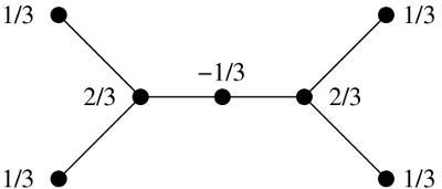
Let’s have an example: once more, the 5-cycle $C_5$.

• A weighting on the adjacency matrix $A_G$ of a graph $G$ is a way of assigning to each vertex $x$ a real number $w(x)$, such that $\sum_{y: y \text{ adjacent to } x} w(y) = 1$ for each vertex $x$. There’s a unique weighting on $C_5$, giving weight $1/3$ to each vertex. The magnitude is the sum of the weights, so $\left|C_5\right| = 5/3 = 1.66\ldots$.

• The maximum diversity is the independence number: $D_{max}(C_5) = \alpha(C_5) = 2$.

• The Shannon capacity is $\Theta(C_5) = \sqrt{5} = 2.23\ldots$.

• The Lovász number is the same: $\vartheta(C_5) = \sqrt{5} = 2.23\ldots$.

It’s immediately clear that unlike the Lovász number, magnitude is not a helpful upper bound for the Shannon capacity — it’s not an upper bound at all. Indeed, it’s not even an upper bound for the independence number.

So for $G = C_5$,

$$\left|G\right| \leq D_{max}(G) = \alpha(G) \leq \Theta(G) \leq \vartheta(G).$$

The equality and the second and third inequalities are true for all $G$. I don’t know whether the first inequality is true in general— that is, whether the magnitude of a graph is always less than or equal to its maximum diversity. Or if not, is it at least true that $\left|G\right| \leq \Theta(G)$ for all $G$? Again, I don’t know.

Nor do I know where to go from here. Most of my understanding of magnitude and maximum diversity comes from the context of metric spaces. (For a finite metric space $X$, one uses the similarity matrix $Z$ given by $Z_{x y} = e^{-d(x, y)}$.) For subspaces of Euclidean space, maximum diversity is always less than or equal to magnitude — which is the opposite way round from what we just saw. That’s because in Euclidean space, passing to a subspace always decreases the magnitude, and by the principle I mentioned earlier, the maximum diversity of a space is equal to the magnitude of some subspace.

Mark Meckes has done a great deal to illuminate the concept of maximum diversity and its relationship to magnitude, putting it into a satisfying analytical setting, not just for finite spaces but also for compact subspaces of Euclidean space (and more generally, so-called spaces of negative type). You can read about this in Positive definite metric spaces and a new paper — Edit: out now! Magnitude, diversity, capacities, and dimensions of metric spaces. But all that’s in a geometrical context quite unlike the graph-theoretic world.

I don’t know whether these ideas lead anywhere interesting. The root of the problem is that I don’t understand much about the magnitude of (the adjacency matrix of) a graph. If you have any insights or observations, I’d very much like to hear them.