The n-Category Café

Enriched Categories

Normally, we like to think that there is a set $\mathcal{C}(A, B)$ of arrows between any two objects $A$ and $B$ in a category $\mathcal{C}$. Composition then can be packaged up into a function $\mathcal{C}(A, B) \times \mathcal{C}(B, C) \to \mathcal{C}(A, C)$, satisfying an associativity condition. The identity is an element of $\mathcal{C}(A, A)$, which we can associate with a function $1 \to \mathcal{C}(A, A)$ from the terminal object. Note that $1$ acts as a unit (up to isomorphism) for the cartesian product $\times$.

We can abstract the structure of $1$ and $\times$ needed to express the axioms of a category as above and describe it in any category. We don’t need the limit properties of $1$ and $\times$ to describe a category, so we won’t keep them as part of our abstraction. What we are left with is the notion of a monoidal category, a category equipped with an object $1$ (not necessarily terminal!) and a binary operation $\otimes$ which satisfy the axioms of a monoid up to isomorphism (and then some conditions on those isomorphisms). We’ll ask for our monoidal categories to be symmetric, meaning that $A \otimes B \cong B \otimes A$ (in a nice, natural way).

Expressing the axioms of a category in more general monoidal categories $(\mathcal{V}, \otimes, 1)$ gives us categories enriched in $\mathcal{V}$. We call $\mathcal{V}$ the base category. Here are some examples of enriched categories over various bases to keep in mind:

• ($\mathcal{V} = \text{Set}$) If the base category is the category of sets, then our categories are the ones we are familiar with. In particular, all the other sorts of base categories are presumed to be enriched over the category of sets.
• ($\mathcal{V} = \text{Ab}$) If the base category is abelian groups with their tensor product $\otimes$ (and unit $\Z$), then we can add and subtract arrows $A \to B$ in our categories. Furthermore, composition is bilinear with regards to the addition of arrows. An example of these sorts of categories are the categories of modules over a ring with the addition of arrows taken pointwise.
• ($\mathcal{V} = \text{Top}$) If our base category is topological spaces with its cartesian structure, then we have a full space of arrows between any two objects in our categories. Furthermore, composition is continuous.
• ($\mathcal{V} = \{\false \to \true\}$) If our base category is the truth values with “and” as their product and $\true$ as the unit, then our categories are just orders. The object of arrows $\mathcal{C}(A, B)$ is a truth value, and we interpret it as the truth of the statement that $A$ is at most $B$. For more on category theory over the truth values, check out Simon Willerton’s post on this blog!
• ($\mathcal{V} = [0,\infty]$) This example is rather surprising. If our base category is the non-negative real numbers, including infinity, with the ‘greater than’ ordering and ‘plus’ as its monoidal structure, then our categories are directed metric spaces. The object of arrows $\mathcal{C}(A, B)$ is a non-negative real number which we interpret as the distance from $A$ to $B$. William Lawvere was the first to write about this in his paper Metric Spaces, Generalized Logic, and Closed Categories

In order for the theory of enriched categories to work out nicely, we will ask for two further conditions on our base categories: closure and cocompleteness. A monoidal category $\mathcal{V}$ is closed if the functors $- \otimes A$ have right adjoints $\mathcal{V}(A, -)$. These objects $\mathcal{V}(A, B)$ therefore behave as an internal hom, an object consisting of morphisms from $A$ to $B$.

To see why, let’s briefly introduce the notation $\mathcal{V}_0(A, B)$ to denote the set of morphisms from $A$ to $B$ in $\mathcal{V}$. Note that $1 \otimes A \cong A$ (by assumption), so $\mathcal{V}_0(1 \otimes A, B) \cong \mathcal{V}_0(A, B)$. But by definition, then $\mathcal{V}_0(A, B) \cong \mathcal{V}_0(1, \mathcal{V}(A, B))$; in other words, the set of morphisms from $A$ to $B$ in $\mathcal{V}$ is the same as the set of points $1 \to \mathcal{V}(A, B)$.

Being cocomplete means that we can glue the objects of our base together. We use this all the time behind the scenes in category theory. Note that since $- \otimes A$ is a left adjoint, it commutes with colimits; this is like the distribution of multiplication over addition.

From now on, all our base categories will be assumed to be symmetric monoidal closed and cocomplete.

* Remark * Even though we started with the monoidal structure $\otimes$ above, sometimes it is more natural to start with the internal hom and then define the monoidal structure to be its left adjoint. For example, it’s pretty easy to see how to endow the set of homomorphisms between two abelian groups with the structure of an abelian group: just add pointwise! Then, we can define the tensor product $A \otimes B$ to be that abelian group which represents $\text{Ab}(A, \text{Ab}(B, C))$. This shows that maps out of $A \otimes B$ must be bilinear; they are linear first in $A$, and then in $B$.

Weighted Limits and Colimits

Enriched category theory (over a general base $\mathcal{V}$) plays out much like usual category theory over the sets, so long as everything is proved in a nicely categorical manner. One major difference, however, is the behavior of (co)limits.

In the category of sets, functions are determined by their actions on points. But in more general base categories, morphisms (by which I mean points of the set of morphisms) may be equal on points (by which I mean morphisms from the monoidal unit $1$) but differ in other ways. For this reason, we need to update our notion of (co)limit for the enriched context by letting the cones have a fatter sort of shape. We call this enriched notion of (co)limit a weighted (co)limit. Kelly calls it an indexed (co)limit. (I would like to thank Pierre for the following discussion about defining cones in the enriched context)

The limit of a diagram $D : \mathcal{D} \to \mathcal{C}$ is more correctly a limiting cone; the object that we call the limit sits atop a “wireframe” cone that projects down toward the diagram. Usually, we define a cone slickly as a natural transformation $\Delta C \to D$ from a constant diagram at an object $C$ in $\mathcal{C}$ to the diagram $D$. The universal property of the limit then looks like this: $$\mathcal{C}(C, \text{lim} D) \cong \mathcal{C}^{\mathcal{D}}(\Delta C, D).$$

To define the constant diagram, we collapse all the arrows of $\mathcal{D}$ onto the identity of $C$; this requires being able to “forget” the data in an object of our base. Arrow theoretically, we have $\mathcal{D}(i, j) \to 1 \to \mathcal{C}(C,C)$ with the first arrow being the unique map guaranteed by the universal property of the terminal object. But in the enriched context, our monoidal unit $1$ may not be terminal, so we won’t be able to do this in general! We need to rephrase our definition of the limit.

We can do this by working with diagrams in $\mathcal{V}$ (where we have access to the objects $\mathcal{C}(A, B)$), instead of of diagrams in $\mathcal{C}$. $$\mathcal{C}(C, \lim D) \cong \mathcal{V}^{\mathcal{D}}(1, \mathcal{C}(C, D(-)).$$ This says that maps into the limit (in $\mathcal{C}(C, \lim D)$) correspond to cones over the diagram (points of $\mathcal{C}(C, D(-))$ in the category of diagrams in the base). Saying that the cone has a “wireframe” shape just means that we are looking at points $1 \to \mathcal{C}(C, D(-))$. For a given object $i$ in $\mathcal{D}$, we then get a point $1 \to \mathcal{C}(C, D_i)$, a single morphism extending from $C$ to $D_i$. But points are often not sensitive enough over a general base, so for a nicely enriched notion of limit, we will need to consider more general figures $W_i \to \mathcal{C}(C, D_i)$. Here, $W : \mathcal{D} \to \mathcal{V}$ is a functor of weights, and the universal property of the weighted limit is $$\mathcal{C}(C, \lim_W D) \cong \mathcal{V}^{\mathcal{D}}(W(-), \mathcal{C}(C, D(-)).$$

Weighted colimits are defined by the dual formula, with morphisms coming out of the diagram. Conical (“wireframe”) (co)limits are just weighted limits whose weights are constant at the monoidal identity.

Over a general base, we can consider a weighted limit of a particularly simple sort. Let $\mathcal{D}$ be the category with a single object and its identity arrow, so that a diagram $D : \mathcal{D} \to \mathcal{C}$ is just an object of $\mathcal{C}$. Then, given a weight $W : \mathcal{D} \to \mathcal{V}$, the universal property says $$\mathcal{C}(C, D^W) \cong \mathcal{V}^{\mathcal{D}}(W, \mathcal{C}(C, D)),$$ where I have taken the liberty of renaming the limit $D^W$ because this is precisely the universal property of the power! If sets are our base, then $D^W$ is a product of $W$ copies of the object $D$, which justifies the name “power”.

Dually, the copower $W \cdot D$ is the weighted colimit of the above data, and over sets it is the coproduct of $W$ copies of $D$. But beware; we need the weights to be contravariant for a colimit, so that $W(-)$ and $\mathcal{C}(D(-), C)$ have the same variance.

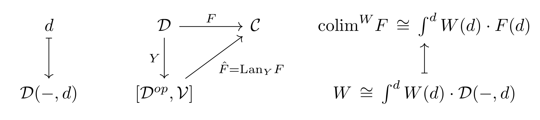
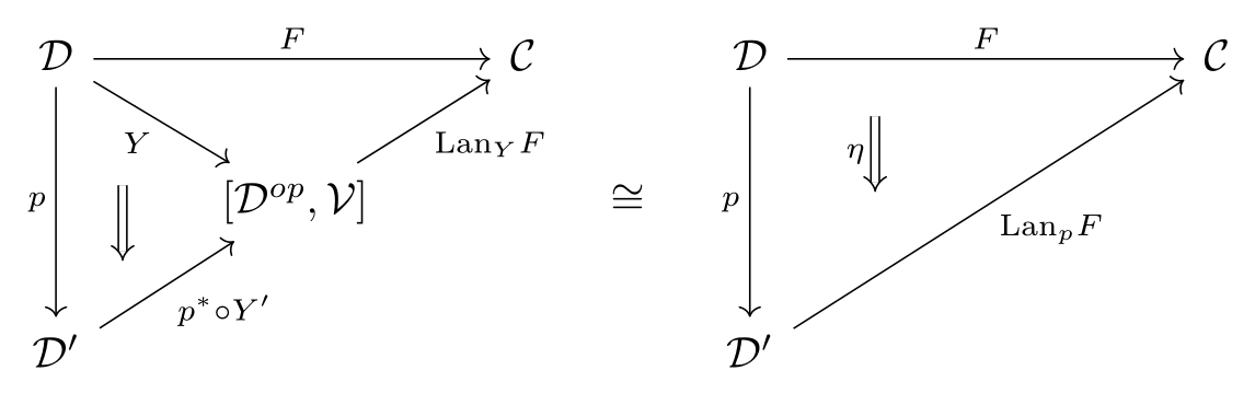
Taking weighted (co)limits is in fact functorial in the weights. For colimits this relationship is covariant; for limits it is contravariant. This means that for suitably cocomplete $\mathcal{C}$, we get a functor $\mathcal{V}^{\mathcal{D}^{\text{op}}} \to \mathcal{C}$ for any diagram $D : \mathcal{D} \to \mathcal{C}$ which sends a weight to the colimit of $D$ weighted by it. This operation corresponds to left Kan extension of the diagram along the Yoneda embedding. Dually, right Kan extension can be expressed by taking weighted limits. As a corollary, we see that all concepts are weighted (co)limits.

An Example: Limits are Weighted Limits!

Here’s a very cool example of a weighted limit which finally lets us tie categorical limits to their analytic analogs. Recall that if our base is the non-negative real numbers $[0, \infty]$, ordered by $\geq$ and with monoidal structure $+$ and $0$, then categories are directed metric spaces. A functor is then a map which does not increase distance between points. We’ll show that certain weighted limits of sequences are their limits in the analytic sense.

Consider the discrete metric space $\mathcal{D}$ whose points are the natural numbers and where $\mathcal{D}(n, m) = \infty$ for all $n$ and $m$. A diagram $D : \mathcal{D} \to \mathcal{C}$ is therefore simply a sequence in $\mathcal{C}$; since the distance between any two points of $\mathcal{D}$ is infinite, no function can increase distance, so all functions are functors. Suppose we have a decreasing sequence $W : \mathcal{D} \to [0,\infty]$ whose limit, in the analytic sense, is $0$. The universal property of the limit of $D$, weighted by $W$, is then $$\mathcal{C}(C, \lim_W D) \cong [0,\infty]^{\mathcal{D}}(W(-), \mathcal{C}(C, D(-))),$$ which, with a little jiggling of the abstract definitions into their specializations, becomes $$\mathcal{C}(C, \lim_W D) = \text{sup}_{i \in \mathcal{D}}(\mathcal{C}(C, D_i) - W-i).$$ In particular, $$0 = \mathcal{C}(\lim_W D, \lim_W D) = \text{sup}_{i \in \mathcal{D}}(\mathcal{C}(\lim_W D, D_i) - W_i),$$ which shows that the sequence $D$ approaches $\lim_W D$ in the analytic sense! (That subtraction is the internal hom in $[0, \infty]$. It is truncated, so if it were going to be negative it gets set to $0$.) It can, in fact, be shown that a sequence is Cauchy if and only if such a weight exists; see this very cool paper by Rutten for details.

If you enjoyed this example, check out Simon Willerton’s posts about the Legendre-Fenchel transform on this very blog!

The $\mathcal{V}$ Point of View

As a general motto, when we are working over a base category $\mathcal{V}$, the category $\mathcal{V}$, as a category enriched over itself, “thinks” it is the category of sets. By this I mean that if we work only using the tensor and internal hom of $\mathcal{V}$ to discuss things, then many of the peculiar features that the category of sets has as a (set-)category, the category $\mathcal{V}$ has as a $\mathcal{V}$-category. For example:

• As I mentioned above, functions in the category of sets are determined by their actions on points. This is not true of a general base category if we think of it as a category over sets. But, if we think of $\mathcal{V}$ as a category over itself, then we have that $\mathcal{V}(1, X) \cong X$ naturally in $X$. By $\mathcal{V}(1, X)$ here I mean the internal hom of $\mathcal{V}$. This means that from the $\mathcal{V}$-point of view, a morphism is determined by its action on points.
• We can build on the last bullet point. We like to think of sets as totally discrete; they are, in fact, all disjoint unions of points. This totally fails in a general base category if we think of it as a category over the sets; for example, not all abelian groups are free (that is, not all abelian groups are coproducts of the monoidal unit $\Z$). But, if we work over a base category $\mathcal{V}$, then “disjoint union” should really mean “copower”. In $\mathcal{V}$, the copower is just the tensor product and therefore $V \cdot 1 \cong V$. So, from the $\mathcal{V}$-point of view, every object is a sum of points.

Check out the next post to see some of the cool things you can do from the $\mathcal{V}$ point of view!