The n-Category Café

In late 1940s, just as Feynman was developing his diagrams for processes in particle physics, Eilenberg and Mac Lane initiated their work on category theory. Over the subsequent decades, and especially in the work of Joyal and Street in the 1980s, it became clear that these developments were profoundly linked: monoidal categories have a precise graphical representation in terms of string diagrams, and conversely monoidal categories provide an algebraic foundation for the intuitions behind Feynman diagrams. The key insight is the use of categories where morphisms describe physical processes, rather than structure-preserving maps between mathematical objects.

In work on fundamental physics, the cutting edge has moved from categories to higher categories. But the same techniques have filtered into more immediate applications, particularly in computation and quantum computation. Our paper is part of a new program of applying string diagrams to engineering, with the aim of giving diverse diagram languages a unified foundation based on category theory.

Indeed, even before physicists began using Feynman diagrams, various branches of engineering were using diagrams that in retrospect are closely related. Foremost among these are the ubiquitous electrical circuit diagrams. Although less well-known, similar diagrams are used to describe networks consisting of mechanical, hydraulic, thermodynamic and chemical systems. Further work, pioneered in particular by Forrester and Odum, applies similar diagrammatic methods to biology, ecology, and economics.

As discussed in detail by Olsen, Paynter and others, there are mathematically precise analogies between these different systems. In each case, the system’s state is described by variables that come in pairs, with one variable in each pair playing the role of ‘displacement’ and the other playing the role of ‘momentum’. In engineering, the time derivatives of these variables are sometimes called ‘flow’ and ‘effort’.

	displacement:    $q$	flow:      $\dot q$	momentum:      $p$	effort:           $\dot p$
Mechanics: translation	position	velocity	momentum	force
Mechanics: rotation	angle	angular velocity	angular momentum	torque
Electronics	charge	current	flux linkage	voltage
Hydraulics	volume	flow	pressure momentum	pressure
Thermal Physics	entropy	entropy flow	temperature momentum	temperature
Chemistry	moles	molar flow	chemical momentum	chemical potential

In classical mechanics, this pairing of variables is well understood using symplectic geometry. Thus, any mathematical formulation of the diagrams used to describe networks in engineering needs to take symplectic geometry as well as category theory into account.

While diagrams of networks have been independently introduced in many disciplines, we do not expect formalizing these diagrams to immediately help the practitioners of these disciplines. At first the flow of information will mainly go in the other direction: by translating ideas from these disciplines into the language of modern mathematics, we can provide mathematicians with food for thought and interesting new problems to solve. We hope that in the long run mathematicians can return the favor by bringing new insights to the table.

Although we keep the broad applicability of network diagrams in the back of our minds, our paper talks in terms of electrical circuits, for the sake of familiarity. We also consider a somewhat limited class of circuits. We only study circuits built from ‘passive’ components: that is, those that do not produce energy. Thus, we exclude batteries and current sources. We only consider components that respond linearly to an applied voltage. Thus, we exclude components such as nonlinear resistors or diodes. Finally, we only consider components with one input and one output, so that a circuit can be described as a graph with edges labeled by components. Thus, we also exclude transformers. The most familiar components our framework covers are linear resistors, capacitors and inductors.

While we want to expand our scope in future work, the class of circuits made from these components has appealing mathematical properties, and is worthy of deep study. Indeed, these circuits has been studied intensively for many decades by electrical engineers. Even circuits made exclusively of resistors have inspired work by mathematicians of the caliber of Weyl and Smale!

Our work relies on this research. All we are adding is an emphasis on symplectic geometry and an explicitly ‘compositional’ framework, which clarifies the way a larger circuit can be built from smaller pieces. This is where monoidal categories become important: the main operations for building circuits from pieces are composition and tensoring. Our strategy is most easily illustrated for circuits made of linear resistors. Such a resistor dissipates power, turning useful energy into heat at a rate determined by the voltage across the resistor. However, a remarkable fact is that a circuit made of these resistors always acts to minimize the power dissipated this way. This ‘principle of minimum power’ can be seen as the reason symplectic geometry becomes important in understanding circuits made of resistors, just as the principle of least action leads to the role of symplectic geometry in classical mechanics.

Here is a circuit made of linear resistors:

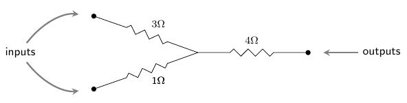
The wiggly lines are resistors, and their resistances are written beside them: for example, $3\Omega$ means 3 ohms, an ‘ohm’ being a unit of resistance. To formalize this, define a circuit of linear resistors to consist of:

• a set $N$ of nodes,
• a set $E$ of edges,
• maps $s,t : E \to N$ sending each edge to its source and target node,
• a map $r: E \to (0,\infty)$ specifying the resistance of the resistor labelling each edge,
• maps $i : X \to N,$ $o : Y \to N$ specifying the inputs and outputs of the circuit.

When we run electric current through such a circuit, each node $n \in N$ gets a potential $\phi(n).$ The voltage across an edge $e \in E$ is defined as the change in potential as we move from to the source of $e$ to its target, $\phi(t(e)) - \phi(s(e)).$ The power dissipated by the resistor on this edge is then

$$\displaystyle{ \frac{1}{r(e)}\big(\phi(t(e))-\phi(s(e))\big)^2 }$$

The total power dissipated by the circuit is therefore twice

$$\displaystyle{ P(\phi) = \frac{1}{2}\sum_{e \in E} \frac{1}{r(e)}\big(\phi(t(e))-\phi(s(e))\big)^2 }$$

The factor of $\frac{1}{2}$ is convenient in some later calculations.

Note that $P$ is a nonnegative quadratic form on the vector space $\mathbb{R}^N.$ However, not every nonnegative definite quadratic form on $\mathbb{R}^N$ arises in this way from some circuit of linear resistors with $N$ as its set of nodes. The quadratic forms that do arise are called Dirichlet forms. They have been extensively investigated, and they play a major role in our work.

We write

$$\partial N = i(X) \cup o(Y)$$

for the set of terminals: that is, nodes corresponding to inputs or outputs. The principle of minimum power says that if we fix the potential at the terminals, the circuit will choose the potential at other nodes to minimize the total power dissipated. An element $\psi$ of the vector space $\mathbb{R}^{\partial N}$ assigns a potential to each terminal. Thus, if we fix $\psi,$ the total power dissipated will be twice

$$Q(\psi) = \min_{\substack{ \phi \in \mathbb{R}^N \\ \phi\vert_{\partial N} = \psi}} \; P(\phi)$$

The function $Q : \mathbb{R}^{\partial N} \to \mathbb{R}$ is again a Dirichlet form. We call it the power functional of the circuit.

Now, suppose we are unable to see the internal workings of a circuit, and can only observe its ‘external behavior’: that is, the potentials at its terminals and the currents flowing into or out of these terminals. Remarkably, this behavior is completely determined by the power functional $Q.$ The reason is that the current at any terminal can be obtained by differentiating $Q$ with respect to the potential at this terminal, and relations of this form are all the relations that hold between potentials and currents at the terminals.

The Laplace transform allows us to generalize this immediately to circuits that can also contain linear inductors and capacitors, simply by changing the field we work over, replacing $\mathbb{R}$ by the field $\mathbb{R}(s)$ of rational functions of a single real variable, and talking of impedance where we previously talked of resistance. We obtain a category ${Circ}$ where an object is a finite set, a morphism $f : X \to Y$ is a circuit with input set $X$ and output set $Y,$ and composition is given by identifying the outputs of one circuit with the inputs of the next, and taking the resulting union of labelled graphs. Each such circuit gives rise to a Dirichlet form, now defined over $\mathbb{R}(s),$ and this Dirichlet form completely describes the externally observable behavior of the circuit.

We can take equivalence classes of circuits, where two circuits count as the same if they have the same Dirichlet form. We wish for these equivalence classes of circuits to form a category. Although there is a notion of composition for Dirichlet forms, we find that it lacks identity morphisms or, equivalently, it lacks morphisms representing ideal wires of zero impedance. To address this we turn to Lagrangian subspaces of symplectic vector spaces. These generalize quadratic forms via the map

$$\Big(Q: \mathbb{F}^{\partial N} \to \mathbb{F}\Big) \mapsto$$

$${Graph}(d Q) = \{(\psi, d Q_\psi) \mid \psi \in \mathbb{F}^{\partial N} \} \; \subseteq \; \mathbb{F}^{\partial N} \oplus (\mathbb{F}^{\partial N})^\ast$$

taking a quadratic form $Q$ on the vector space $\mathbb{F}^{\partial N}$ over the field $\mathbb{F}$ to the graph of its differential $d Q.$ Here we think of the symplectic vector space $\mathbb{F}^{\partial N} \oplus (\mathbb{F}^{\partial N})^\ast$ as the state space of the circuit, and the subspace ${Graph}(d Q)$ as the subspace of attainable states, with $\psi \in \mathbb{F}^{\partial N}$ describing the potentials at the terminals, and $d Q_\psi \in (\mathbb{F}^{\partial N})^\ast$ the currents.

This construction is well-known in classical mechanics, where the principle of least action plays a role analogous to that of the principle of minimum power here. The set of Lagrangian subspaces is actually an algebraic variety, the Lagrangian Grassmannian, which serves as a compactification of the space of quadratic forms. The Lagrangian Grassmannian has already played a role in Sabot’s work on circuits made of resistors. For us, its importance it that we can find identity morphisms for the composition of Dirichlet forms by taking circuits made of parallel resistors and letting their resistances tend to zero: the limit is not a Dirichlet form, but it exists in the Lagrangian Grassmannian.

Indeed, there exists a category ${LagrRel}$ with finite dimensional symplectic vector spaces as objects and Lagrangian relations as morphisms: that is, linear relations from $V$ to $W$ that are given by Lagrangian subspaces of $\overline{V} \oplus W,$ where $\overline{V}$ is the symplectic vector space conjugate to $V$—that is, with the sign of the symplectic structure switched.

To move from the Lagrangian subspace defined by the graph of the differential of the power functional to a morphism in the category ${LagrRel}$ — that is, to a Lagrangian relation — we must treat seriously the input and output functions of the circuit. These express the circuit as built upon a cospan:

Applicable far more broadly than for our formalization of circuits, cospans model systems with two ‘ends’, an input and output end, albeit without any connotation of directionality: we might just as well exchange the role of the inputs and outputs by taking the mirror image of the above diagram. The role of the input and output functions, as we have discussed, is to mark the terminals we may glue onto the terminals of another circuit, and the pushout of cospans gives formal precision to this gluing construction.

One upshot of this cospan framework is that we may consider circuits with elements of $N$ that are both inputs and outputs, such as this one:

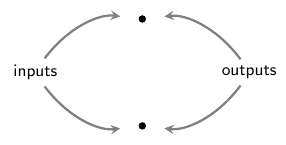
This corresponds to the identity morphism on the finite set with two elements. Another is that some points may be considered an input or output multiple times, like here:

This lets to connect two distinct outputs to the above double input.

Given a set $X$ of inputs or outputs, we understand the electrical behavior on this set by considering the symplectic vector space $\mathbb{F}^X \oplus {(\mathbb{F}^X)}^\ast,$ the direct sum of the space $\mathbb{F}^X$ of potentials and the space ${(\mathbb{F}^X)}^\ast$ of currents at these points. A Lagrangian relation specifies which states of the output space $\mathbb{F}^Y \oplus {(\mathbb{F}^Y)}^\ast$ are allowed for each state of the input space $\mathbb{F}^X \oplus {(\mathbb{F}^X)}^\ast.$ Turning the Lagrangian subspace ${Graph}(d Q)$ of a circuit into this information requires that we understand the ‘symplectification’

$$S f: \mathbb{F}^B \oplus {(\mathbb{F}^B)}^\ast \to \mathbb{F}^A \oplus {(\mathbb{F}^A)}^\ast$$ and ‘twisted symplectification’

$$S^t f: \mathbb{F}^B \oplus {(\mathbb{F}^B)}^\ast \to \overline{\mathbb{F}^A \oplus {(\mathbb{F}^A)}^\ast}$$

of a function $f: A \to B$ between finite sets.

Symplectification and twisted symplectification are contravariant functors from $Finset$ to $LagrRel$. We need to understand how these apply to the input and output functions with codomain restricted to $\partial N$; abusing notation, we write these as $i: X \to \partial N$ and $o: Y \to \partial N.$

The symplectification $S f$ is a Lagrangian relation, and the catch phrase is that it ‘copies voltages’ and ‘splits currents’. More precisely, for any given potential-current pair $(\psi,\iota)$ in $\mathbb{F}^B \oplus {(\mathbb{F}^B)}^\ast,$ its image under $S f$ consists of all elements of $(\psi', \iota')$ in $\mathbb{F}^A \oplus {(\mathbb{F}^A)}^\ast$ such that the potential at $a \in A$ is equal to the potential at $f(a) \in B,$ and such that, for each fixed $b \in B,$ collectively the currents at the $a \in f^{-1}(b)$ sum to the current at $b.$ We use the symplectification $S o$ of the output function to relate the state on $\partial N$ to that on the outputs $Y.$

As our current framework is set up to report the current out of each node, to describe input currents we define the twisted symplectification:

$$S^t f: \mathbb{F}^B \oplus {(\mathbb{F}^B)}^\ast \to \overline{\mathbb{F}^A \oplus {(\mathbb{F}^A)}^\ast}$$

almost identically to the above, except that we flip the sign of the currents $\iota' \in (\mathbb{F}^A)^\ast.$ This again gives a Lagrangian relation. We use the twisted symplectification $S^t i$ of the input function to relate the state on $\partial N$ to that on the inputs.

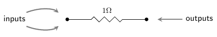
The Lagrangian relation corresponding to a circuit then comprises exactly a list of the potential-current pairs that are possible electrical states of the inputs and outputs of the circuit. In doing so, it identifies distinct circuits. A simple example of this is the identification of a single 2-ohm resistor:

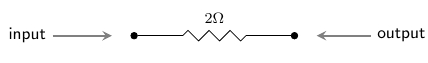
with two 1-ohm resistors in series:

Our inability to access the internal workings of a circuit in this representation inspires us to call this process black boxing: you should imagine encasing the circuit in an opaque black box, leaving only the terminals accessible. Fortunately, this information is enough to completely characterize the external behavior of a circuit, including how it interacts when connected with other circuits!

Put more precisely, the black boxing process is functorial: we can compute the black-boxed version of a circuit made of parts by computing the black-boxed versions of the parts and then composing them. In fact we shall prove that ${Circ}$ and ${LagrRel}$ are dagger compact categories, and the black box functor preserves all this extra structure:

Theorem. There exists a symmetric monoidal dagger functor, the black box functor

$$\blacksquare: {Circ} \to {LagrRel}$$

mapping a finite set $X$ to the symplectic vector space $\mathbb{F}^X \oplus (\mathbb{F}^X)^\ast$ it generates, and a circuit $\big((N,E,s,t,r),i,o\big)$ to the Lagrangian relation

$$\bigcup_{v \in {Graph}(d Q)} S^t i(v) \times S o(v) \subseteq \overline{\mathbb{F}^X \oplus (\mathbb{F}^X)^\ast} \oplus \mathbb{F}^Y \oplus (\mathbb{F}^Y)^\ast$$

where $Q$ is the circuit’s power functional.

The goal of this paper is to prove and explain this result. The proof is more tricky than one might first expect, but our approach involves concepts that should be useful throughout the study of networks, such as ‘decorated cospans’ and ‘corelations’.

Give it a read, and let us know if you have questions or find mistakes!