The n-Category Café

Despite my ultimate aim of studying biological and ecological networks, I decided to start by clarifying the math of networks that appear in chemistry and engineering, since these are simpler, better understood, useful in their own right, and probably a good warmup for the grander goal. I’ve been working with Brendan Fong on electrical ciruits, and with Jason Erbele on control theory. Let me talk about this paper:

• John Baez and Jason Erbele, Categories in control.

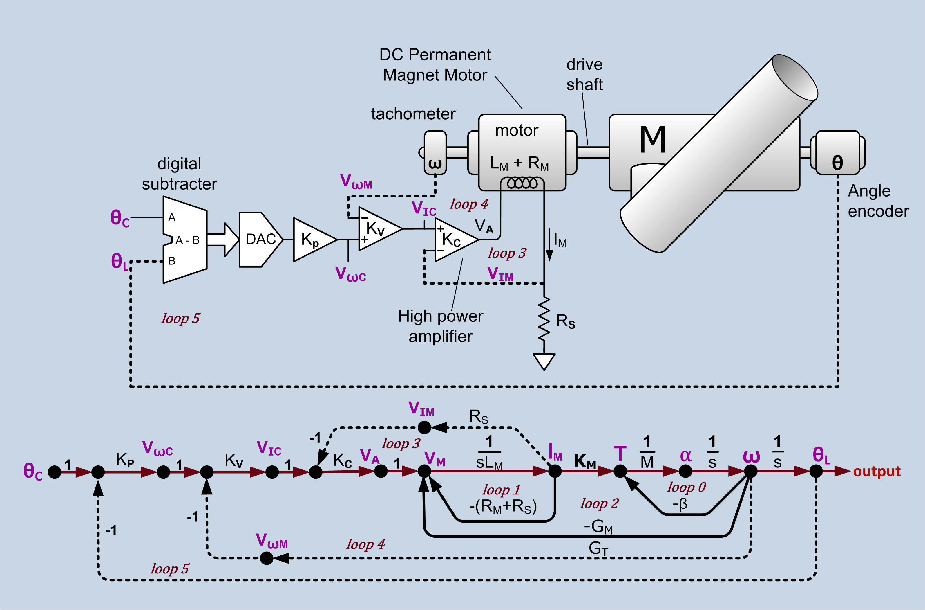
Control theory is the branch of engineering that focuses on manipulating open systems—systems with inputs and outputs—to achieve desired goals. In control theory, signal-flow diagrams are used to describe linear ways of manipulating signals, for example smooth real-valued functions of time. Here’s a real-world example; click the picture for more details:

For a category theorist, at least, it is natural to treat signal-flow diagrams as string diagrams in a symmetric monoidal category. This forces some small changes of perspective, which I’ll explain, but more important is the question: which symmetric monoidal category?

We argue that the answer is: the category $\mathrm{FinRel}_k$ of finite-dimensional vector spaces over a certain field $k,$ but with linear relations rather than linear maps as morphisms, and direct sum rather than tensor product providing the symmetric monoidal structure. We use the field $k = \mathbb{R}(s)$ consisting of rational functions in one real variable $s.$ This variable has the meaning of differentation. A linear relation from $k^m$ to $k^n$ is thus a system of linear constant-coefficient ordinary differential equations relating $m$ ‘input’ signals and $n$ ‘output’ signals.

Our main goal in this paper is to provide a complete ‘generators and relations’ picture of this symmetric monoidal category, with the generators being familiar components of signal-flow diagrams. It turns out that the answer has an intriguing but mysterious connection to ideas that are familiar in the diagrammatic approach to quantum theory! Quantum theory also involves linear algebra, but it uses linear maps between Hilbert spaces as morphisms, and the tensor product of Hilbert spaces provides the symmetric monoidal structure.

We hope that the category-theoretic viewpoint on signal-flow diagrams will shed new light on control theory. However, in this paper we only lay the groundwork.

Signal flow diagrams

There are several basic operations that one wants to perform when manipulating signals. The simplest is multiplying a signal by a scalar. A signal can be amplified by a constant factor:

$$f \mapsto cf$$

where $c \in \mathbb{R}.$ We can write this as a string diagram:

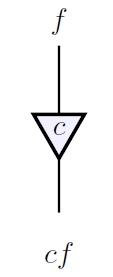
Here the labels $f$ and $c f$ on top and bottom are just for explanatory purposes and not really part of the diagram. Control theorists often draw arrows on the wires, but this is unnecessary from the string diagram perspective. Arrows on wires are useful to distinguish objects from their duals, but ultimately we will obtain a compact closed category where each object is its own dual, so the arrows can be dropped. What we really need is for the box denoting scalar multiplication to have a clearly defined input and output. This is why we draw it as a triangle. Control theorists often use a rectangle or circle, using arrows on wires to indicate which carries the input $f$ and which the output $c f.$

A signal can also be integrated with respect to the time variable:

$$f \mapsto \int f$$

Mathematicians typically take differentiation as fundamental, but engineers sometimes prefer integration, because it is more robust against small perturbations. In the end it will not matter much here. We can again draw integration as a string diagram:

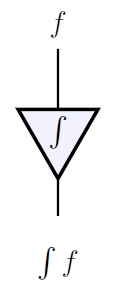
Since this looks like the diagram for scalar multiplication, it is natural to extend $\mathbb{R}$ to $\mathbb{R}(s),$ the field of rational functions of a variable $s$ which stands for differentiation. Then differentiation becomes a special case of scalar multiplication, namely multiplication by $s,$ and integration becomes multiplication by $1/s.$ Engineers accomplish the same effect with Laplace transforms, since differentiating a signal $f$ is equivalent to multiplying its Laplace transform

$$\displaystyle{ (\mathcal{L}f)(s) = \int_0^\infty f(t) e^{-st} \,dt }$$

by the variable $s.$ Another option is to use the Fourier transform: differentiating $f$ is equivalent to multiplying its Fourier transform

$$\displaystyle{ (\mathcal{F}f)(\omega) = \int_{-\infty}^\infty f(t) e^{-i\omega t}\, dt }$$

by $-i\omega.$ Of course, the function $f$ needs to be sufficiently well-behaved to justify calculations involving its Laplace or Fourier transform. At a more basic level, it also requires some work to treat integration as the two-sided inverse of differentiation. Engineers do this by considering signals that vanish for $t < 0,$ and choosing the antiderivative that vanishes under the same condition. Luckily all these issues can be side-stepped in a formal treatment of signal-flow diagrams: we can simply treat signals as living in an unspecified vector space over the field $\mathbb{R}(s).$ The field $\mathbb{C}(s)$ would work just as well, and control theory relies heavily on complex analysis. In our paper we work over an arbitrary field $k.$

The simplest possible signal processor is a rock, which takes the 'input' given by the force $F$ on the rock and produces as 'output' the rock's position $q.$ Thanks to Newton's second law $F=ma,$ we can describe this using a signal-flow diagram:

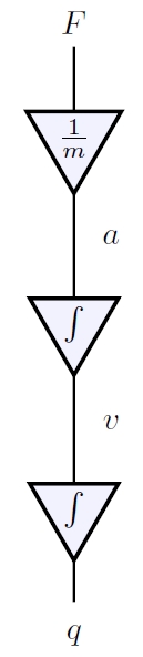
Here composition of morphisms is drawn in the usual way, by attaching the output wire of one morphism to the input wire of the next.

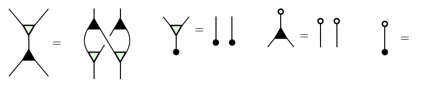
To build more interesting machines we need more building blocks, such as addition:

$$+ : (f,g) \mapsto f + g$$

and duplication:

$$\Delta : f \mapsto (f,f)$$

When these linear maps are written as matrices, their matrices are transposes of each other. This is reflected in the string diagrams for addition and duplication:

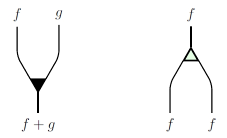
The second is essentially an upside-down version of the first. However, we draw addition as a dark triangle and duplication as a light one because we will later want another way to ‘turn addition upside-down’ that does not give duplication. As an added bonus, a light upside-down triangle resembles the Greek letter $\Delta,$ the usual symbol for duplication.

While they are typically not considered worthy of mention in control theory, for completeness we must include two other building blocks. One is the zero map from the zero-dimensional vector space $\{0\}$ to our field $k,$ which we denote as $0$ and draw as follows:

The other is the zero map from $k$ to $\{0\},$ sometimes called ‘deletion’, which we denote as $!$ and draw thus:

Just as the matrices for addition and duplication are transposes of each other, so are the matrices for zero and deletion, though they are rather degenerate, being $1 \times 0$ and $0 \times 1$ matrices, respectively. Addition and zero make $k$ into a commutative monoid, meaning that the following relations hold:

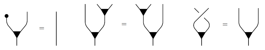
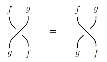
The equation at right is the commutative law, and the crossing of strands is the braiding:

$$B : (f,g) \mapsto (g,f)$$

by which we switch two signals. In fact this braiding is a symmetry, so it does not matter which strand goes over which:

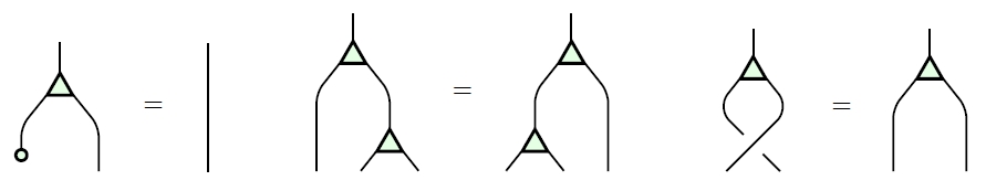
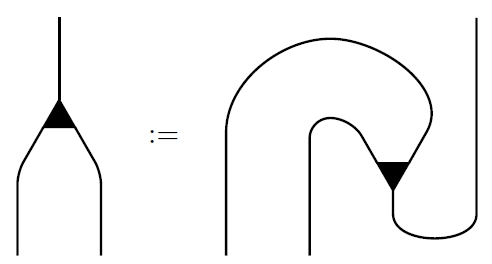
Dually, duplication and deletion make $k$ into a cocommutative comonoid. This means that if we reflect the equations obeyed by addition and zero across the horizontal axis and turn dark operations into light ones, we obtain another set of valid equations:

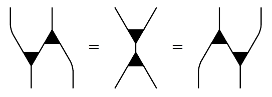
There are also relations between the monoid and comonoid operations. For example, adding two signals and then duplicating the result gives the same output as duplicating each signal and then adding the results:

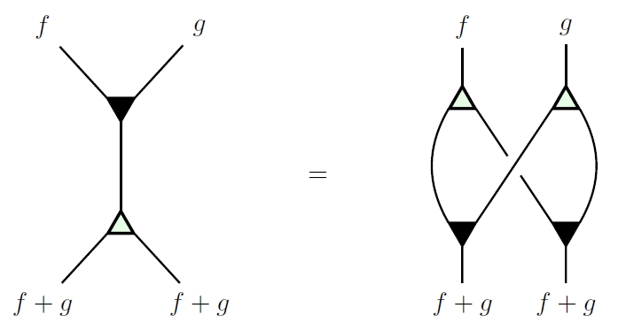
This diagram is familiar in the theory of Hopf algebras, or more generally bialgebras. Here it is an example of the fact that the monoid operations on $k$ are comonoid homomorphisms—or equivalently, the comonoid operations are monoid homomorphisms.

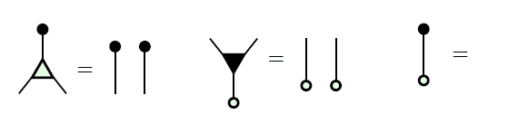
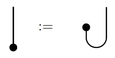
We summarize this situation by saying that $k$ is a bimonoid. These are all the bimonoid laws, drawn as diagrams:

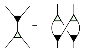
The last equation means we can actually make the diagram at left disappear, since it equals the identity morphism on the 0-dimensional vector space, which is drawn as nothing.

So far all our string diagrams denote linear maps. We can treat these as morphisms in the category $\mathrm{FinVect}_k,$ where objects are finite-dimensional vector spaces over a field $k$ and morphisms are linear maps. This category is equivalent to the category where the only objects are vector spaces $k^n$ for $n \ge 0,$ and then morphisms can be seen as $n \times m$ matrices. The space of signals is a vector space $V$ over $k$ which may not be finite-dimensional, but this does not cause a problem: an $n \times m$ matrix with entries in $k$ still defines a linear map from $V^n$ to $V^m$ in a functorial way.

In applications of string diagrams to quantum theory, we make $\mathrm{FinVect}_k$ into a symmetric monoidal category using the tensor product of vector spaces. In control theory, we instead make $\mathrm{FinVect}_k$ into a symmetric monoidal category using the direct sum of vector spaces. In Lemma 1 of our paper we prove that for any field $k,$ $\mathrm{FinVect}_k$ with direct sum is generated as a symmetric monoidal category by the one object $k$ together with these morphisms:

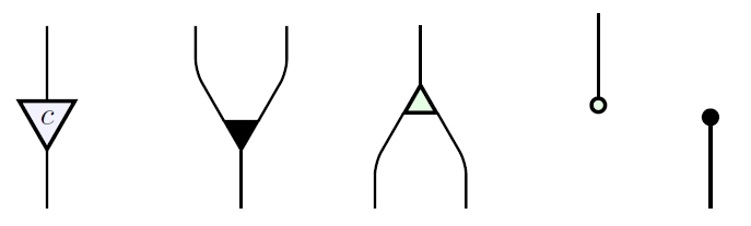
where $c \in k$ is arbitrary.

However, these generating morphisms obey some unexpected relations! For example, we have:

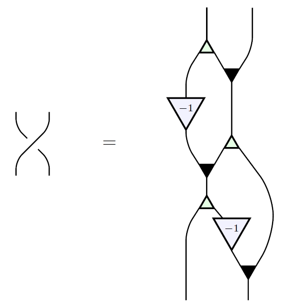
Thus, it is important to find a complete set of relations obeyed by these generating morphisms, thus obtaining a presentation of $\mathrm{FinVect}_k$ as a symmetric monoidal category. We do this in Theorem 2. In brief, these relations say:

(1) $(k, +, 0, \Delta, !)$ is a bicommutative bimonoid;

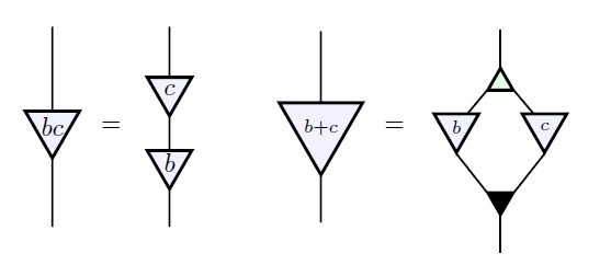
(2) the rig operations of $k$ can be recovered from the generating morphisms;

(3) all the generating morphisms commute with scalar multiplication.

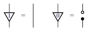
Here item (2) means that $+, \cdot, 0$ and $1$ in the field $k$ can be expressed in terms of signal-flow diagrams as follows:

Multiplicative inverses cannot be so expressed, so our signal-flow diagrams so far do not know that $k$ is a field. Additive inverses also cannot be expressed in this way. So, we expect that a version of Theorem 2 will hold whenever $k$ is a mere rig: that is, a ‘ring without negatives’, like the natural numbers. The one change is that instead of working with vector spaces, we should work with finitely presented free $k$-modules.

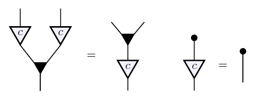
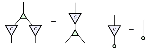
Item (3), the fact that all our generating morphisms commute with scalar multiplication, amounts to these diagrammatic equations:

While Theorem 2 is a step towards understanding the category-theoretic underpinnings of control theory, it does not treat signal-flow diagrams that include ‘feedback’. Feedback is one of the most fundamental concepts in control theory because a control system without feedback may be highly sensitive to disturbances or unmodeled behavior. Feedback allows these uncontrolled behaviors to be mollified. As a string diagram, a basic feedback system might look schematically like this:

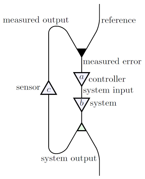
The user inputs a ‘reference’ signal, which is fed into a controller, whose output is fed into a system, which control theorists call a ‘plant’, which in turn produces its own output. But then the system’s output is duplicated, and one copy is fed into a sensor, whose output is added (or if we prefer, subtracted) from the reference signal.

In string diagrams—unlike in the usual thinking on control theory—it is essential to be able to read any diagram from top to bottom as a composite of tensor products of generating morphisms. Thus, to incorporate the idea of feedback, we need two more generating morphisms. These are the ‘cup’:

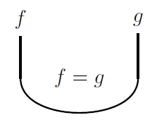
and ‘cap’:

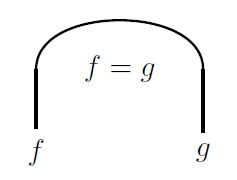
These are not maps: they are relations. The cup imposes the relation that its two inputs be equal, while the cap does the same for its two outputs. This is a way of describing how a signal flows around a bend in a wire.

To make this precise, we use a category called $\mathrm{FinRel}_k.$ An object of this category is a finite-dimensional vector space over $k,$ while a morphism from $U$ to $V,$ denoted $L : U \rightharpoonup V,$ is a linear relation, meaning a linear subspace

$$L \subseteq U \oplus V$$

In particular, when $k = \mathbb{R}(s),$ a linear relation $L : k^m \to k^n$ is just an arbitrary system of constant-coefficient linear ordinary differential equations relating $m$ input variables and $n$ output variables.

Since the direct sum $U \oplus V$ is also the cartesian product of $U$ and $V,$ a linear relation is indeed a relation in the usual sense, but with the property that if $u \in U$ is related to $v \in V$ and $u' \in U$ is related to $v' \in V$ then $c u + c'u'$ is related to $c v + c'v'$ whenever $c,c' \in k.$

We compose linear relations $L : U \rightharpoonup V$ and $L' : V \rightharpoonup W$ as follows:

$$L'L = \{(u,w) \colon \; \exists\; v \in V \;\; (u,v) \in L \; and \; (v,w) \in L'\}$$

Any linear map $f : U \to V$ gives a linear relation $F : U \rightharpoonup V,$ namely the graph of that map:

$$F = \{ (u,f(u)) : u \in U \}$$

Composing linear maps thus becomes a special case of composing linear relations, so $\mathrm{FinVect}_k$ becomes a subcategory of $\mathrm{FinRel}_k.$ Furthermore, we can make $\mathrm{FinRel}_k$ into a monoidal category using direct sums, and it becomes symmetric monoidal using the braiding already present in $\mathrm{FinVect}_k.$

In these terms, the cup is the linear relation

$$\cup : k^2 \rightharpoonup \{0\}$$

given by

$$\cup \; = \; \{ (x,x,0) : x \in k \} \; \subseteq \; k^2 \oplus \{0\}$$

while the cap is the linear relation

$$\cap : \{0\} \rightharpoonup k^2$$

given by

$$\cap \; = \; \{ (0,x,x) : x \in k \} \; \subseteq \; \{0\} \oplus k^2$$

These obey the zigzag relations:

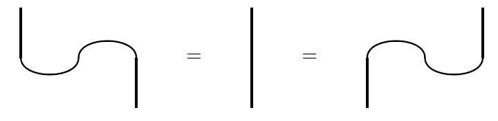
Thus, they make $\mathrm{FinRel}_k$ into a compact closed category where $k,$ and thus every object, is its own dual.

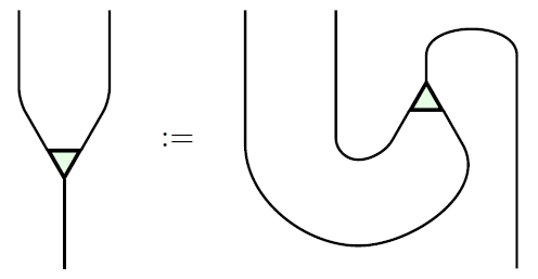
Besides feedback, one of the things that make the cap and cup useful is that they allow any morphism $L : U \rightharpoonup V$ to be ‘plugged in backwards’ and thus ‘turned around’. For instance, turning around integration:

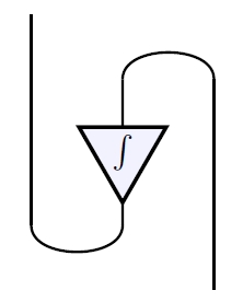
we obtain differentiation. In general, using caps and cups we can turn around any linear relation $L : U \rightharpoonup V$ and obtain a linear relation $L^\dagger : V \rightharpoonup U,$ called the adjoint of $L,$ which turns out to given by

$L^\dagger = \{(v,u) : (u,v) \in L \}$

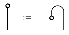
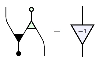
For example, if $c \in k$ is nonzero, the adjoint of scalar multiplication by $c$ is multiplication by $c^{-1}$:

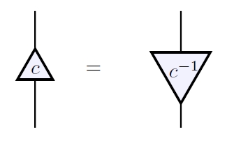
Thus, caps and cups allow us to express multiplicative inverses in terms of signal-flow diagrams! One might think that a problem arises when when $c = 0,$ but no: the adjoint of scalar multiplication by $0$ is

$\{(0,x) : x \in k \} \subseteq k \oplus k$

In Lemma 3 we show that $\mathrm{FinRel}_k$ is generated, as a symmetric monoidal category, by these morphisms:

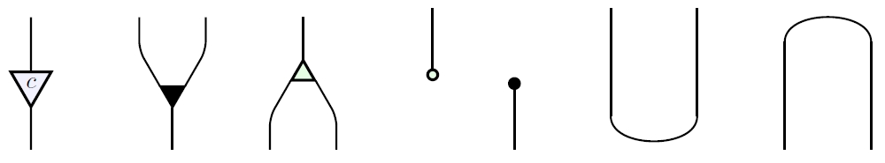
where $c \in k$ is arbitrary.

In Theorem 4 we find a complete set of relations obeyed by these generating morphisms,thus giving a presentation of $\mathrm{FinRel}_k$ as a symmetric monoidal category. To describe these relations, it is useful to work with adjoints of the generating morphisms. We have already seen that the adjoint of scalar multiplication by $c$ is scalar multiplication by $c^{-1},$ except when $c = 0.$ Taking adjoints of the other four generating morphisms of $\mathrm{FinVect}_k,$ we obtain four important but perhaps unfamiliar linear relations. We draw these as ‘turned around’ versions of the original generating morphisms:

• Coaddition is a linear relation from $k$ to $k^2$ that holds when the two outputs sum to the input:

$+^\dagger : k \rightharpoonup k^2$

$+^\dagger = \{(x,y,z) : \; x = y + z \} \subseteq k \oplus k^2$

• Cozero is a linear relation from $k$ to $\{0\}$ that holds when the input is zero:

$0^\dagger : k \rightharpoonup \{0\}$

$0^\dagger = \{ (0,0)\} \subseteq k \oplus \{0\}$

• Coduplication is a linear relation from $k^2$ to $k$ that holds when the two inputs both equal the output:

$\Delta^\dagger : k^2 \rightharpoonup k$

$\Delta^\dagger = \{(x,y,z) : \; x = y = z \} \subseteq k^2 \oplus k$

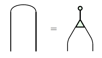
• Codeletion is a linear relation from $\{0\}$ to $k$ that holds always:

$!^\dagger : \{0\} \rightharpoonup k$

$!^\dagger = \{(0,x) \} \subseteq \{0\} \oplus k$

Since $+^\dagger,0^\dagger,\Delta^\dagger$ and $!^\dagger$ automatically obey turned-around versions of the relations obeyed by $+,0,\Delta$ and $!,$ we see that $k$ acquires a second bicommutative bimonoid structure when considered as an object in $\mathrm{FinRel}_k.$

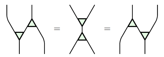
Moreover, the four dark operations make $k$ into a Frobenius monoid. This means that $(k,+,0)$ is a monoid, $(k,+^\dagger, 0^\dagger)$ is a comonoid, and the Frobenius relation holds:

All three expressions in this equation are linear relations saying that the sum of the two inputs equal the sum of the two outputs.

The operation sending each linear relation to its adjoint extends to a contravariant functor

$$\dagger : \mathrm{FinRel}_k \to \mathrm{FinRel}_k$$

which obeys a list of properties that are summarized by saying that $\mathrm{FinRel}_k$ is a †-compact category. Because two of the operations in the Frobenius monoid $(k, +,0,+^\dagger,0^\dagger)$ are adjoints of the other two, it is a †-Frobenius monoid.

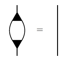
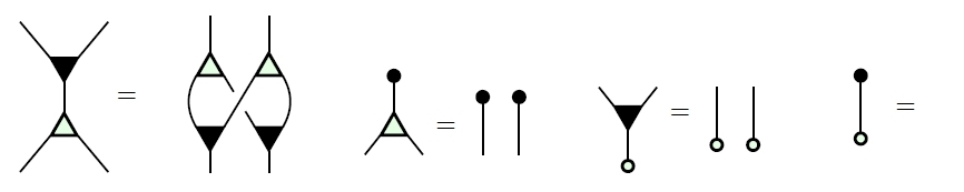
This Frobenius monoid is also special, meaning that comultiplication (in this case $+^\dagger$) followed by multiplication (in this case $+$) equals the identity:

This Frobenius monoid is also commutative—and cocommutative, but for Frobenius monoids this follows from commutativity.

Starting around 2008, commutative special †-Frobenius monoids have become important in the categorical foundations of quantum theory, where they can be understood as ‘classical structures’ for quantum systems. The category $\mathrm{FinHilb}$ of finite-dimensional Hilbert spaces and linear maps is a †-compact category, where any linear map $f : H \to K$ has an adjoint $f^\dagger : K \to H$ given by

$\langle f^\dagger \phi, \psi \rangle = \langle \phi, f \psi \rangle$

for all $\psi \in H, \phi \in K .$ A commutative special †-Frobenius monoid in $\mathrm{FinHilb}$ is then the same as a Hilbert space with a chosen orthonormal basis. The reason is that given an orthonormal basis $\psi_i$ for a finite-dimensional Hilbert space $H,$ we can make $H$ into a commutative special †-Frobenius monoid with multiplication $m : H \otimes H \to H$ given by

$$m (\psi_i \otimes \psi_j ) = \left\{ \begin{array}{cl} \psi_i & i = j \\ 0 & i \ne j \end{array}\right.$$

and unit $i : \mathbb{C} \to H$ given by

$$i(1) = \sum_i \psi_i$$

The comultiplication $m^\dagger$ duplicates basis states:

$$m^\dagger(\psi_i) = \psi_i \otimes \psi_i$$

Conversely, any commutative special †-Frobenius monoid in $\mathrm{FinHilb}$ arises this way.

Considerably earlier, around 1995, commutative Frobenius monoids were recognized as important in topological quantum field theory. The reason, ultimately, is that the free symmetric monoidal category on a commutative Frobenius monoid is $2\mathrm{Cob},$ the category with 2-dimensional oriented cobordisms as morphisms. But the free symmetric monoidal category on a commutative special Frobenius monoid was worked out even earlier: it is the category with finite sets as objects, where a morphism $f : X \to Y$ is an isomorphism class of cospans

$$X \longrightarrow S \longleftarrow Y$$

This category can be made into a †-compact category in an obvious way, and then the 1-element set becomes a commutative special †-Frobenius monoid.

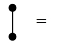
For all these reasons, it is interesting to find a commutative special †-Frobenius monoid lurking at the heart of control theory! However, the Frobenius monoid here has yet another property, which is more unusual. Namely, the unit $0 : \{0\} \rightharpoonup k$ followed by the counit $0^\dagger : k \rightharpoonup \{0\}$ is the identity:

We call a special Frobenius monoid that also obeys this extra law extra-special. One can check that the free symmetric monoidal category on a commutative extra-special Frobenius monoid is the category with finite sets as objects, where a morphism $f : X \to Y$ is an equivalence relation on the disjoint union $X \sqcup Y,$ and we compose $f : X \to Y$ and $g : Y \to Z$ by letting $f$ and $g$ generate an equivalence relation on $X \sqcup Y \sqcup Z$ and then restricting this to $X \sqcup Z.$

As if this were not enough, the light operations share many properties with the dark ones. In particular, these operations make $k$ into a commutative extra-special †-Frobenius monoid in a second way. In summary:

• $(k, +, 0, \Delta, !)$ is a bicommutative bimonoid;

• $(k, \Delta^\dagger, !^\dagger, +^\dagger, 0^\dagger)$ is a bicommutative bimonoid;

• $(k, +, 0, +^\dagger, 0^\dagger)$ is a commutative extra-special †-Frobenius monoid;

• $(k, \Delta^\dagger, !^\dagger, \Delta, !)$ is a commutative extra-special †-Frobenius monoid.

It should be no surprise that with all these structures built in, signal-flow diagrams are a powerful method of designing processes.

However, it is surprising that most of these structures are present in a seemingly very different context: the so-called ZX calculus, a diagrammatic formalism for working with complementary observables in quantum theory. This arises naturally when one has an $n$-dimensional Hilbert space $H$ with two orthonormal bases $\psi_i, \phi_i$ that are mutually unbiased, meaning that

$$|\langle \psi_i, \phi_j \rangle|^2 = \displaystyle{\frac{1}{n}}$$

for all $1 \le i, j \le n.$ Each orthonormal basis makes $H$ into commutative special †-Frobenius monoid in $\mathrm{FinHilb}.$ Moreover, the multiplication and unit of either one of these Frobenius monoids fits together with the comultiplication and counit of the other to form a bicommutative bimonoid. So, we have all the structure present in the list above—except that these Frobenius monoids are only extra-special if $H$ is 1-dimensional.

The field $k$ is also a 1-dimensional vector space, but this is a red herring: in $\mathrm{FinRel}_k$ every finite-dimensional vector space naturally acquires all four structures listed above, since addition, zero, duplication and deletion are well-defined and obey all the relations we have discussed. Jason and I focus on $k$ in our paper simply because it generates all the objects $\mathrm{FinRel}_k$ via direct sum.

Finally, in $\mathrm{FinRel}_k$ the cap and cup are related to the light and dark operations as follows:

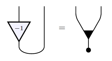
Note the curious factor of $-1$ in the second equation, which breaks some of the symmetry we have seen so far. This equation says that two elements $x, y \in k$ sum to zero if and only if $-x = y.$ Using the zigzag relations, the two equations above give

We thus see that in $\mathrm{FinRel}_k,$ both additive and multiplicative inverses can be expressed in terms of the generating morphisms used in signal-flow diagrams.

Theorem 4 of our paper gives a presentation of $\mathrm{FinRel}_k$ based on the ideas just discussed. Briefly, it says that $\mathrm{FinRel}_k$ is equivalent to the symmetric monoidal category generated by an object $k$ and these morphisms:

• addition $+: k^2 \rightharpoonup k$ • zero $0 : \{0\} \rightharpoonup k$ • duplication $\Delta: k\rightharpoonup k^2$ • deletion $! : k \rightharpoonup 0$ • scalar multiplication $c: k\rightharpoonup k$ for any $c\in k$ • cup $\cup : k^2 \rightharpoonup \{0\}$ • cap $\cap : \{0\} \rightharpoonup k^2$

obeying these relations:

(1) $(k, +, 0, \Delta, !)$ is a bicommutative bimonoid;

(2) $\cap$ and $\cup$ obey the zigzag equations;

(3) $(k, +, 0, +^\dagger, 0^\dagger)$ is a commutative extra-special †-Frobenius monoid;

(4) $(k, \Delta^\dagger, !^\dagger, \Delta, !)$ is a commutative extra-special †-Frobenius monoid;

(5) the field operations of $k$ can be recovered from the generating morphisms;

(6) the generating morphisms (1)-(4) commute with scalar multiplication.

Note that item (2) makes $\mathrm{FinRel}_k$ into a †-compact category, allowing us to mention the adjoints of generating morphisms in the subsequent relations. Item (5) means that $+, \cdot, 0, 1$ and also additive and multiplicative inverses in the field $k$ can be expressed in terms of signal-flow diagrams in the manner we have explained.

So, we have a good categorical understanding of the linear algebra used in signal flow diagrams!

Now Jason is moving ahead to apply this to some interesting problems… but that’s another story, for later.