Skew Monoidal Categories Through Triangulations and Examples
Posted by Tom Leinster
.")
Guest post by Thea Li and Pablo S. Ocal
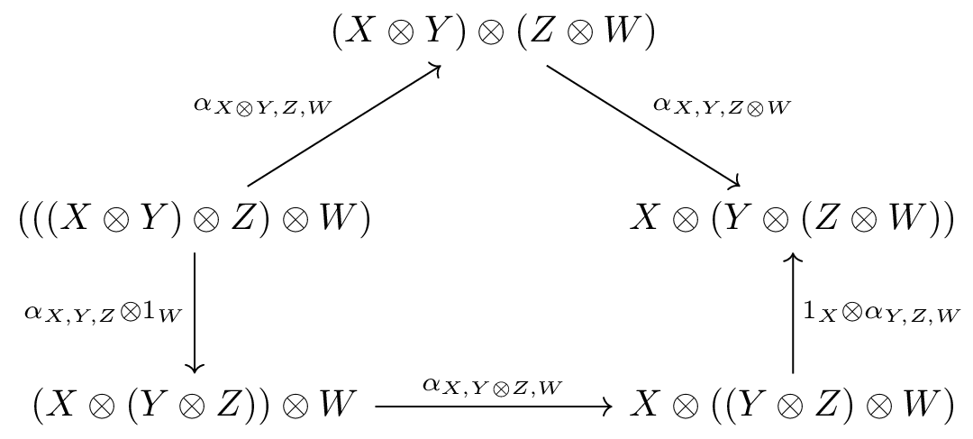
The study of monoidal categories and their applications is an essential part of the research and applications of category theory. However, on occasion the coherence conditions of these categories turns out to be too strong for what one might want (or one might simply be curious as to what happens when their axioms are not all met), leading to the development of various weakenings of these notions. In our case at hand, we consider a weakening in which neither the associator nor the unitors are invertible, which is known as a skew monoidal category. A particularity of these categories is that Mac Lane’s coherence theorem does not apply, whereas there may be parallel arrows formed by structural maps that are not equal.
In this year’s edition of the Adjoint School we covered the paper Triangulations, orientals, and skew monoidal categories by Stephen Lack and Ross Street, in which the authors construct a concrete model of the free skew-monoidal category on a single generating object, from hereon denoted . To do so, one of the main challenges is to encode bracketings in a meaningful way yielding an associator that is not invertible. This lead them to investigate the correspondence between triangulations of polygons and bracketings of finite words, as well as the relationship between the Tamari order, associators, and higher order morphisms between simplexes.
In this blog post we would like to turn our attention to the intuition behind the constructions presented in the paper and illustrate them by working though some examples. It was fascinating to discover that, although the content of the paper is about higher category theory, the technical details essentially boil down to combinatorics.
The definition of skew monoidal category
We begin by recalling the definition of a skew monoidal category. It is possible to make different choices of the direction of the structure maps than the ones presented here, but they will all be equivalent.
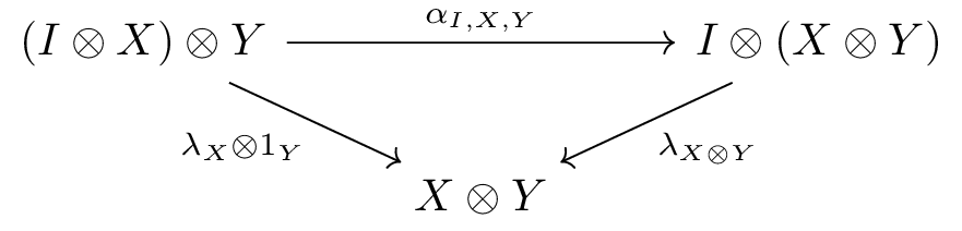
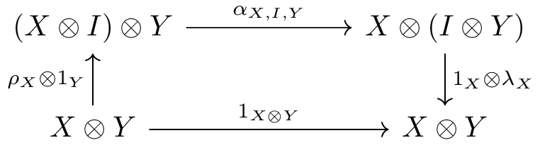
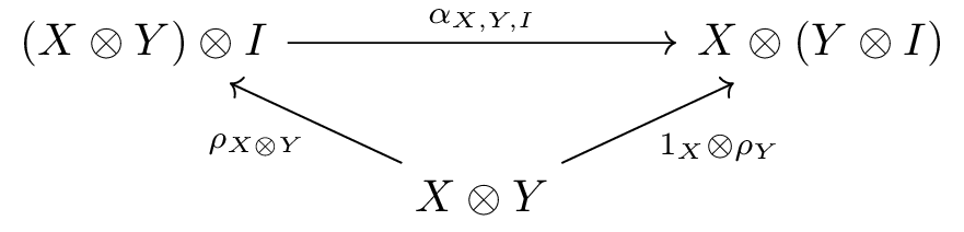
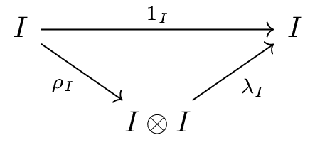
A (left) skew monoidal category is a category equipped with a bifunctor (the tensor product) and an object (the skew unit), together with maps
for each object in . These are subject to the following conditions.
The simplex category and its subcategory
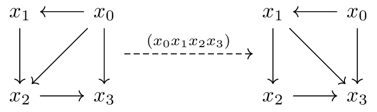
A simple example of a skew monoidal category, that we will base the construction of on, appears as a subcategory of the simplex category equipped with the usual monoidal structure. Recall that has finite ordinals as objects and order preserving functions as morphisms. It is wellknown that we can equip with a symmetric monoidal structure with tensor given by ordinal addition and the empty set as unit. We can define a skew-monoidal structure with the same tensor by restricting ourself to the subcategory of non-empty ordinals and -preserving order preserving functions, , taking as skew-unit. Note that this skew-monoidal category has associativity, as ordinal addition is associative, while the left and right skew-unitors given by and are strict. While this category contains , it is not , though by construction there must be a skew-monoidal functor from to that sends to . It is useful to refer to for intuition about what should be.
We now recall some useful facts about morphisms in . These also hold for morphisms in .
- can be equipped with a 2-categorical structure, where a 2-cell between exists if for all (whence is, in fact, a Poset-enriched category).
- For each finite ordinal and each there is a unique order preserving injection whose image does not contain , and a unique order preserving surjection that identifies and . It turns out that the morphisms in are precisely those generated by these two families of morphisms. This generation is subject to certain rewrite relations giving us a canonical decomposition of a morphism. We note that is the left skew unitor in and is the right skew unitor.
- To be able to properly define morphisms in , we note that a morphism has a right adjoint if and only if it preserves and a left adjoint if and only if it preserves . These are essentially given by: and .
Bracketings, triangulations, and their morphisms
We now describe what will be the associators in .
Triangulations and bracketings
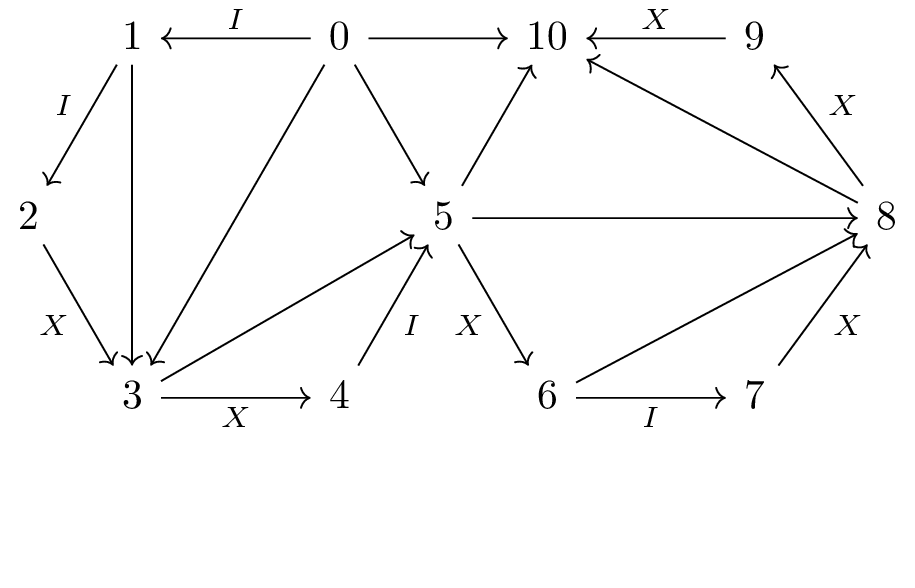
Given an ordinal in , it determines a polygon with sides. A triangulation of this polygon is, intuitively, a way of filling this polygon with triangles in such a way that two distinct triangles only intersect in vertices and edges. For example, a triangulation of is:
Formalizing this is a bit cumbersome.
Definition: A triangle of is a subset with < < . We say that a triangle has left short leg , right short leg , and long leg .
For bookkeeping purposes, it is useful to keep in mind that the domain of an arrow in a triangle should be a strictly smaller natural number than its codomain. This order of the natural numbers will end up inducing a partial order on the set of triangulations of a given polygon.
Definition: A triangulation of an -polygon is a set of triangles of such that:
- Triangles do not share legs with the same name.
- Triangles do not share counterclockwise oriented edges.
- The only long leg that is not short is .
- The only short legs that are not long are for .
Each of these conditions avoids undesirable triangle(s). The first two cases make sure that the triangles within a triangulation do not have intersecting faces, and the last two make sure that the arrows of the triangles within our triangulation point in the correct direction. These four cases correspond to the following configurations.
With this setup, the previous triangulation of is . If we now label the outer edges by for , successive collapsing of the triangulation gives the bracketing of these labels .
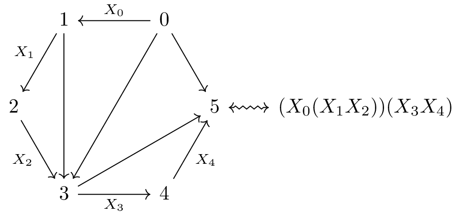
This holds in general. Labeling by the counterclockwise oriented outer edges of the polygon given by , a triangulation of corresponds to a bracketing of the labels. To make this correspondence precise, we first need to determine what exactly is a bracketing. The position of the open brackets will be recorded in the left bracketing function, and the position of the closing brackets will be recorded in the right bracketing function. Namely, given a bracketing, its left bracketing function satisfies that when there is an opening bracket to the left of , and its right bracketing function satisfies that when there is a closing bracket to the right of . Observe that a triangulation of admits distinct labels, so the bracketing functions will have domain and codomain the ordinal . We are now ready.
Definition: A left bracketing function is a morphism of sets such that:
- for all .
- If with then .
- and .
Definition: A right bracketing function is a morphism of sets such that:
- for all .
- If with then .
- and .
Continuing our running example, the left bracketing function of follows.
Moreover, this completely determines the bracketing, there is no need to specify what is the right bracketing function of . Although left and right bracketing functions recorded (a priori) complementary information, the precise definition makes having both redundant. There is, in fact, a bijection between left and right bracketing functions.
Proposition:
- Let be a left bracketing function, then given by < for , and setting and , is a right bracketing function.
- Let be a right bracketing function, then given by < for , and setting and , is a left bracketing function.
- The constructions above are inverses of each other.
We invite the reader to check that the following gives the right bracketing function of .
We can now give the precise statement giving a bijection between triangulations and bracketing functions.
Proposition:
- Let be a left bracketing function, then < < is a triangulation of .
- Let be a triangulation of , then setting , , and for gives a left bracketing function .
- Let be a triangulation of , then setting , , and for gives a right bracketing function .
- corresponds to .
- The constructions above are inverses of each other.
For completeness, let’s summarize the running example we have been exploring. The triangulation can be visualized as

where the bracketing is and the bracketing functions, together with the triangles determining their values, are
An important technical detail is that given a function preserving the order, the top element, and the bottom element (so in particular it has both a left adjoint and a right adjoint ), then: 1. is a left bracketing function for all left bracketing functions , and 2. is a right-bracketing function for all right bracketing functions .
For example, the function has left adjoint and right adjoint It can be checked that is a left bracketing function, with corresponding right bracketing function both of which correspond to the trianglulation of .
Similarly, it can be checked that is a right bracketing function, whose corresponding left bracketing function is and they correspond to the trianglulation of .
Morphisms between triangulations
With all this formalism in place, we can finally define morphisms between triangulations. In the next section, these will play the role of the associators in .
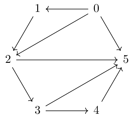
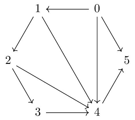
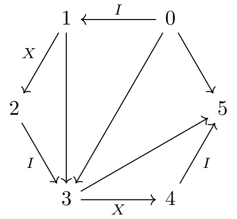
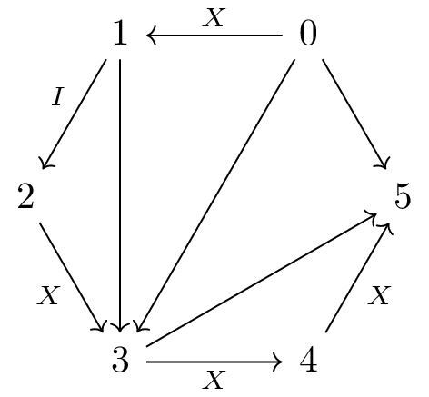
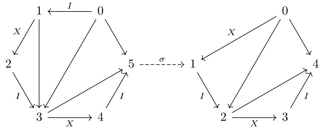
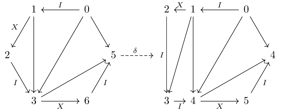
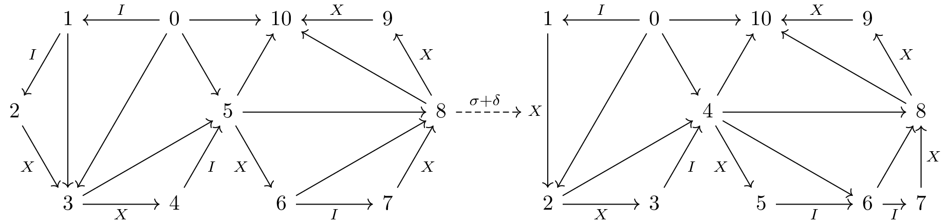
Definition: Let be a triangulation of containing the triangles and . The set is also a triangulation of . The set , also denoted , defines a morphism of triangulations between and .
Locally, the morphism gives a map from the square with vertices and triangulation to the square with vertices and triangulation .
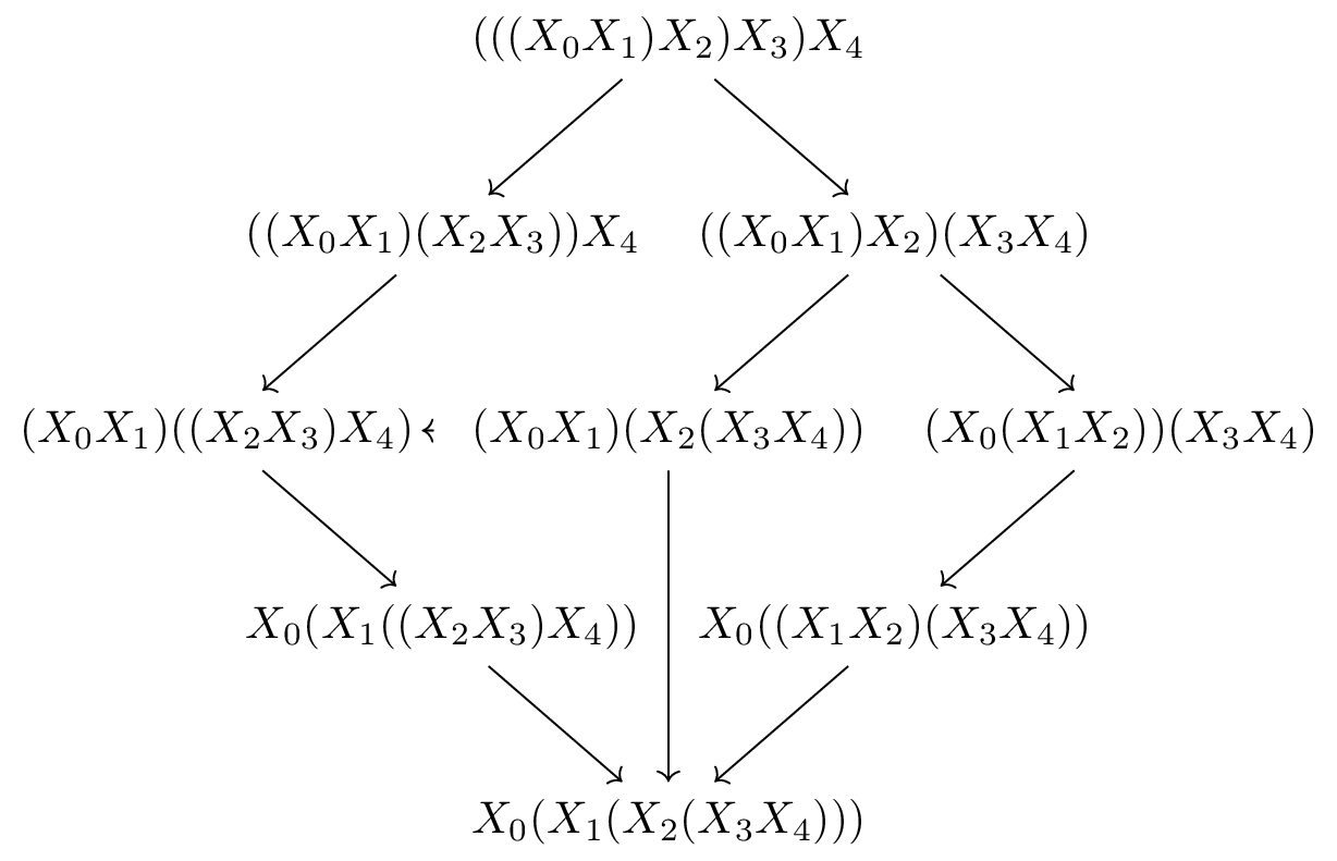
Intuitively, a morphism between two triangulations is a successive exchange of pairs of triangles. Such an exchange essentially results in moving an arrow from the antidiagonal of a square to the diagonal of the same square. The following diagram illustrates two (equal) parallel morphisms from the triangulation to the triangulation , which include a commutative square and two pentagons arising from skew associativity.
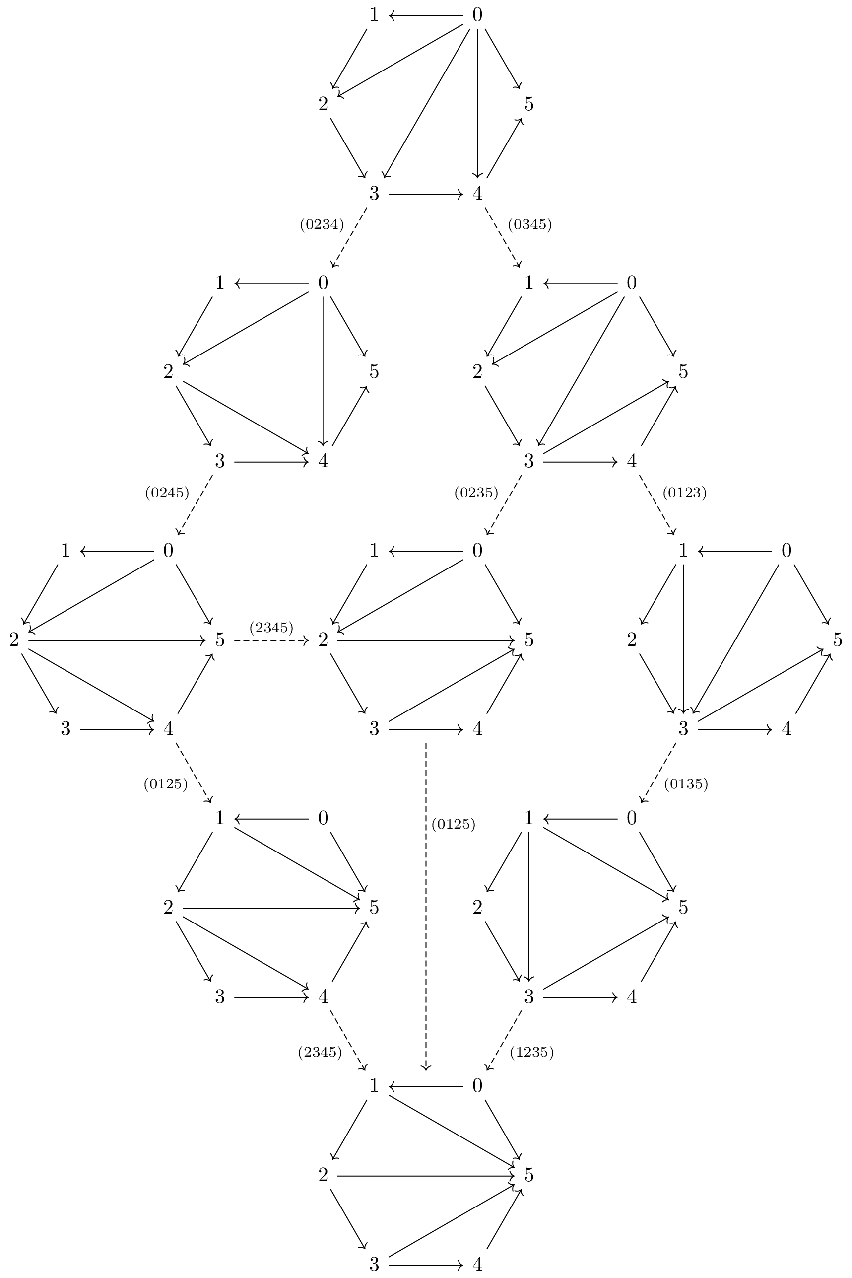
Whenever we have a morphism of triangulations from to , we declare that . This is the aforementioned induced partial order on triangulations. At the level of bracketings, moving from a smaller element to a larger element corresponds to successively associating brackets around the labels from the left to the right. That is, the triangulation corresponding to the bracketing is the smallest element in this order, the triangulation corresponding to the bracketing is the largest element in the partial order, and the morphisms in the previous picture establishes the following poset.
The free skew monoidal category on a single object
We now want to give a proper definition of . Intuitively, has for objects the bracketings of finite products of ’s and skew units ’s, and morphisms generated by the skew associator and skew unitors. To construct , Lack and Street follow this intuitive idea very closely.
The objects
We start by considering what the objects should look like.
Definition: is a discrete category with objects that are tuples , where is a non-empty finite ordinal, is a subset of this ordinal, and a triangulation of .
Intuitively, is giving a polygon, is giving the edges of the polygon where we will have the non-identity object, and is giving a triangulation on the polygon, which we know is comparable to a finite word (or product) consisting of ’s and ’s with a bracketing.
For example we can think about the tuple as the finite word or the following triangulation.

Tensor product
We model the monoidal structure of on the monoidal structure of . The tensor product is thus defined as the following.
Definition: We define a tensor product on objects by where is the disjoint union of and , and is the triangulation associated to the following left bracketing function.
This essentially gives us a “concaternation” or “product” of two objects. For indexes < the tensor product inherits the bracketing of , then setting to gives a bracket around this factor, and when > it inherits the bracketing of . We can see this as “gluing” the second triangulated polygons onto the first.
For example, tensoring
with
gives:
Or seen as the concatenation two finite words, tensoring the object that represents with the one that represents gives us the one that represents .
The morphisms
The morphisms in can be decomposed into three components, a bracket rearranging component (skew associators), a component shrinking skew units ’s to the left (left skew unitor), and a component adding skew units ’s to the right (right skew unitor). We define these in further detail below.
Associators
The most simple component is the one giving us skew associativity.
Definition: Let and be two objects of the same size and the same indexes being ’s. When we say there is a morphism from to . It is the identity on the underlying word, but changes the bracketing from to .
A morphism of this form is called a Tamari morphism. This gives us skew associativity, as per the correspondence between bracketings and triangulations with the Tamari order, is precisely when we can apply skew associators to the bracketing of to get the bracketing of .
Shrink morphisms
For the left skew unitor we define another type of morphism between objects of .
Definition: Let and be two objects in , and let be a surjective order preserving map. Then defines a shrink morphism when
- induces a bijection from to ,
- then ,
- .
Intuitively; 1. says that the morphism preserves the ’s, that is and have the same amount of ’s and they appear in the same place with respect to the bracketings. 3. says that is a “sub-triangulation” of , that is, up to all triangles in appear in . Finally, 2. together with 1. guarantees that we only collapse ’s that are bracketed to the left, namely ’s that appear labeling a right short leg of a triangle.
Recall that in The simplex category and its subcategory we defined a familiy of surjections for each . These are all shrink morphisms, and it is in fact the case that all shrink morphisms can be generated by a composition of ’s.
A shrink morphism precomposed with a Tamari morphism is called an -surjection.
Swell morphisms
We proceed analogously for the right skew unitors.
Definition: Let and be two objects in , and let be an injective left adjoint. Then defines a swell morphism when
- induces a bijection from to ,
- If < , then ,
- .
Again, 1. says that the morphism preserves the ’s, that is and have the same amount of ’s and they appear in the same place with respect to the bracketings. 3. says that is a “sub-triangulation” of , that is, up to all triangles in appear in . Finally, 2. and 1. together say that if an is bracketed towards the right in then it is the image of an that was already bracketed towards the right in .
Recall that in The simplex category and its subcategory we defined a familiy of injections for each , these are all swell morphisms, and it is in fact the case that all swell morphisms can be generated by a composition of ’s.
A swell morphism postcomposed with a Tamari morphism is called an -injection.
Functoriality of tensor
The tensor product on objects defined above can be extended to morphisms by considering the disjoint union of morphisms. This essentially amounts to applying each morphism to the factor or sub-polygon corresponding to each of the objects separately.
For example, the tensor product
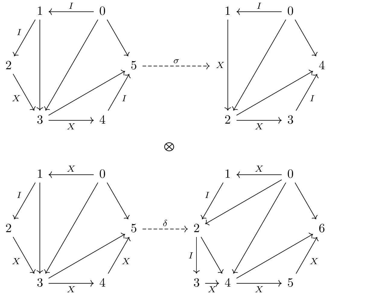
becomes
and its universal property
We now present the long awaited definition of .
Definition: is the category with objects that are tuples , where is a non-empty finite ordinal, is a subset of this ordinal, and a triangulation of . The morphisms are compositions of an -surjection with an -injection.
Theorem: is the free monoidal category over one object.
Corollary: Let be a skew monoidal category. There is a unique strict skew monoidal functor from to sending the generator of to the skew monoidal unit of .