The n-Category Café

Preliminaries

Even though we all have some intuitive grasp of what uncertainty is, providing a formal mathematical framework to represent it has proven to be non-trivial. We may understand uncertainty as the feeling of not being sure if an event will occur in the future. Classically, this feeling is mainly attributed to the lack of knowledge we may have about such an event or phenomenon. Often, this lack of knowledge is a condition from which we cannot escape, and it may preclude us from making reliable statements about the event. Let us think about the case of tossing a coin. If we think in a Newtonian deterministic way, we may think that if we had perfect knowledge about the initial conditions when tossing a coin, this would allow us to know which of the two outcomes will happen.

However, there are numerous unpredictable factors, such as the initial force applied, air currents, the surface it lands on, and microscopic imperfections in the coin itself that prevent us from knowing such initial conditions with infinite accuracy. In particular, at the moment you are throwing the coin you do not know the state of all the actin and myosin proteins in your muscles, which play an important role in your movements and thus in the outcome of the toss. So, even though the laws of physics govern the motion of the coin, its final state will be unpredictable due to the complex interactions of these factors. This forces us to talk about how likely or unlikely an outcome is, leading us to the notion of uncertainty.

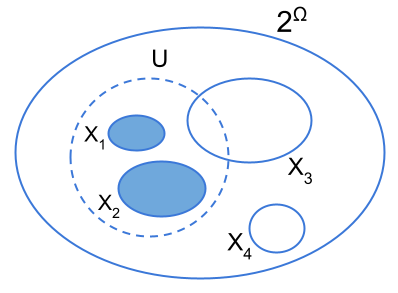
A natural question that arises is how uncertainty can be quantified or, in other words, what is the mathematical framework for representing uncertainty? Usually, we are told that the fundamental tool for analyzing and managing uncertainty is probability, or more specifically, Kolmogorovian probability. However, there are several mathematical representations of uncertainty. Most of these representations, including the classical Kolmogorovian approach, share a couple of key basic ingredients in their way of representing uncertainty. Namely, an outcome space or set of possible worlds $\Omega$, a collection of events or propositions $\mathcal{F}$, and a weight function $f: \mathcal{F} \to [0,1]$. These ingredients will form what we call a coarse-grained representation of uncertainty. To understand each of these concepts we will make use of an example. Suppose that Monica from the TV show Friends spent the whole night cooking a cake she needs to bring to a party the next day. She goes to sleep confident of her hard work and the next day, she wakes up and half of the cake is missing. Immediately, Monica starts building a list of possible suspects who may have eaten the cake. The list includes each of her friends: Rachel $(:= R)$, Chandler $(:= C)$, Joey $(:= J)$, Ross $(:= Ro)$ and Phoebe $(:= P)$ and also possible ”combinations” of these. A possible list of suspects could be $\Omega = \{R, C, Ro, P, RC, RJ, RRo, CJ, CRo, CP, ... , RCJRoP\}$ where, the elements ”containing” more than one suspect, such as $RC, RJ, RRo, RCJRoP$, etc, express the fact that it may be that all these suspects have eaten the cake together. For example, $RC$ express the fact that it was Rachel and Chandler who ate the cake. Each element in $\Omega$ represents a possible scenario or a possible world. One important thing to note is that determining which worlds to include and which to exclude, along with deciding the depth of detail to represent each world, often entails a significant degree of subjective judgment from the agent. For example, if Monica believes in aliens, she might consider it important to include a world in which aliens ate the cake.

Each of the possible worlds may be seen as an event or proposition. However, we may also think of other interesting sets of events such as $\{R,C,J,Ro,P\}$, which express that only one of Monica’s friends is guilty, or the one given by $\{C,J, CJ\}$, which expresses the fact he who eat the cake was either Joey or Chandler, or both together, in contrast with $\{C, J\}$, which states the fact that it was either Joey or Chandler who eat the cake but not both. In particular, we may think about events as sets made of possible worlds. Later, we will require that this collection of events satisfies some closure properties.

Given that Joey, Chandler, and Rachel are the ones who live much closer to Monica and also given that Joey is very fond of food, Monica can differentiate, in likelihood, the elements in the collection of propositions. This differentiation can be done by assigning different ”weights” to each event. The assignment of such weights can be done by means of a weight function, $f$, which assigns to each event a number, the ”weight”, between 0 and 1, which represents the likelihood of such event. Often this weight function is construed as a probability measure. However, there are different ways in which we may think of $f$. In the literature, these other ways of thinking about $f$ are often known by the name of imprecise probabilities.

In this post, we would like to motivate (some of) these other formal approaches to model uncertainty, and discuss some of the limitations that the measure-theoretic probability framework has in modeling uncertainty. Moreover, we would like start the ball rolling on exploring the possibility of studying imprecise probability through a categorical lens. In order to discuss these other formal approaches to model uncertainty we will first start by briefly summarizing what the Kolmogorovian probability theory framework is about.

Probability theory in a nutshell

Measure-theoretic probability is the predominant mathematical framework for understanding uncertainty. We first start with an outcome space $\Omega$, also called sample space. The aforementioned collection of events $\mathcal{F}$ has the structure of a $\sigma$-algebra, that is, a collection of subsets of $\Omega$ which is closed under complementation and under countable unions, that is, if $U_1, U_2, ...$ are in $\mathcal{F}$, then so are $\overline{U_1}, \overline{U_2},...$ and $\cup_i U_i$. In this framework, the function which assigns the likelihood of an event is called a probability measure. Specifically, a probability measure is a set-theoretic function $\mu: \mathcal{F} \to [0,1]$ such that:

$$\mu(\Omega)=1,$$

and

$\mu$ is $\sigma$-additive, i.e., for all countable collections ${\displaystyle \{U_{k}\}_{k=1}^{\infty }}$ of pairwise disjoint sets in $\mathcal{F}$ we have

$$\mu( \bigcup_{k=1}^\infty U_{k}) = \sum_{k=1}^\infty \mu(U_k)$$

These two axioms are usually known as the Kolmogorov axioms. For the sake of simplicity, in the rest of the post, we will consider that our set of outcomes $\Omega$ is finite. So, instead of talking about a $\sigma$-algebra, we can just talk about an algebra over $\Omega$, which means it is enough to consider that the collection is closed under complementation and finite unions and instead of talking about $\sigma$-additivity we will be talking about additivity. In those cases when we have a finite set $\Omega$, we will choose (unless specified) the power set algebra as the algebra over it and we will denote $\mathcal{F}$ as $2^\Omega$. A sample space $\Omega$ together with a $\sigma$-algebra over $\mathcal{F}$, and a probability measure $\mu$ on $\mathcal{F}$ is called a probability space, and it is usually denoted by the triple $(\Omega,\mathcal{F},\mu)$.

Although this mathematical artillery indeed provides us with tools to model uncertainty, there are some vital questions that still need to be answered: what do the numbers we assign to a certain event represent? Where do these numbers come from? And, moreover, why should probabilities have these particular mathematical properties, for example the $\sigma$-additivity? Without answering these questions, assigning probabilities in practical scenarios and interpreting the outcomes derived from this framework will lack clarity.

For now, let’s leave aside the more ”technical” questions and focus on the more ”philosophical” ones. Even though probability theory is the mainstream mathematical theory to represent uncertainty, in the twenty-first century philosophers and mathematicians still have several competing views of what probability is. The two major currents of interpretation are the frequentist and the subjectivist or Bayesian interpretations.

The frequentist theory interprets probability as a certain persistent rate or relative frequency. Specifically, frequentists define the probability of an event as the proportion of times the event occurs in the long run, as the number of trials approaches infinity.While this explanation appears quite natural and intuitive, in practice, you cannot perform an experiment an infinite number of times. Moreover, interpreting probabilities as limiting frequencies can be nonsensical in some scenarios where we have non-repeatable or one-time events. On the other hand, the advocates of the subjective interpretation define probabilities just as numerical values assigned by an individual representing their degree of belief as long as these numerical assignments satisfy the axioms of probability. In both approaches, it can be proved, that the way of interpreting probabilities is compatible with the Kolmogorov axioms (see, for example, section 2.2.1 in [1].

Interpretations of probabilities are usually categorized into two main types: ontological and epistemological. Epistemological interpretations of probability view probability as related to human knowledge or belief. In this perspective, probability represents the extent of knowledge, rational belief, or subjective conviction of a particular human being. In contrast, ontological interpretations of probability consider probability as an inherent aspect of the objective material world, independent of human knowledge or belief.Therefore, we may view the frequentist current as an ontological interpretation whereas the subjective theory may be viewed as an epistemological one. Both points of view of interpreting probabilities, however, are perfectly valid and may be used depending on the particular situation. For example, a doctor’s belief about the probability of a patient having a particular disease based on symptoms, medical history, and diagnostic tests represents an epistemic probability. On the other hand, the probability of a particular isotope of uranium disintegrating in a year represents an objective probability since is related to the spontaneous transformation of the unstable atomic nuclei of the isotope, therefore, the probability exists as a characteristic of the physical world which is independent of human belief. In fact, this probability already existed before humans populated the Earth! Moreover, it seems that the objective interpretation may be more suitable for modeling processes in the framework of parameter estimation theory, while the subjective interpretation may be more useful for modeling decision-making by means of Bayes [2].

What is wrong with probabilities?

As we said before, in order for measure-theoretic probability to be a model of uncertainty it should also answer why probabilities have these specific mathematical properties. In particular we may question the additivity property. Measure-theoretic probability, with its additivity property, models situations of uncertainty where we still know a great deal about the system. Sometimes, however, the uncertainty is so high, or we know so little, that we do not have enough data to construct a probability measure. Let’s see a couple of examples that illustrate this problem.

Example 1: Suppose Alice has a fair coin and proposes the following bet to Bob. If the coin lands tails he must pay her 1€, and if the coin lands heads she must pay him 1€. Since the coin is fair, Bob is neutral about accepting the bet. However, suppose now that Alice has a coin with an unknown bias, and she proposes the same bet. What should Bob choose now? Should Bob refuse to play the game suspecting maybe the worst-case scenario in which Alice is using a coin with two tails?

Since Bob does not know about the bias of the coin, he cannot know the probability behind each of the outcomes. Therefore, his ignorance about the bias may preclude him from making a reasonable bet. This example highlights one of the major challenges of probability theory namely, its inability to effectively represent ignorance since even though we may still want to address this situation mathematically, we lack the required data to establish a probability measure.

Example 2: Imagine you have a bag of 100 gummies. According to the wrapper, $30\%$ of the gummies are red and the rest of them may be either green or yellow. Given that the exact proportion of green and yellow gummies is not known, it seems reasonable to assign a probability of 0.7 to choosing either a green (:= $g$) or a yellow (:= $y$) gummy and a probability of 0.3 to the outcome of choosing a red (:= $r$) gummy. However, what is the probability of choosing just a green (or just a yellow) gummy?

In this example, we have information about the probabilities of a whole proposition $\{g, y\}$, but not about the probabilities of each of its individual outcomes. Let’s take $2^{\Omega_G}$ as the algebra over $\Omega_G= \{r,y,g\}$. This is the ”biggest” algebra we can have so, for sure, if we want to have information about the yellow and green gummies this choice will be helpful. In order to follow the approach of traditional probability theory, we must assign probabilities to all individual outcomes. However, this cannot be done, since we do not have information about how the 0.7 probability is distributed between the green and yellow gummies. Therefore, the fact that an agent is only able to assign probabilities to some sets may be seen as a problem. Of course, there is a natural way to avoid this problem: we can define a smaller algebra which excludes those subsets of the sample space that are ”problematic”. In particular, you may exclude the green and yellow singletons of your algebra, so that you have a probability measure which is consistent with the additivity axiom. However, by implementing this solution we cannot answer our original question either.

Moreover, we may even dare to say that human behaviour is not compatible with assigning probabilities to each of these singletons. Let’s consider the following bets:

1. You get 1€ if the gummy is red, and 0€ otherwise (Fraction of the red gummies: $30\%$).

2. You get 1€ if the gummy is green, and 0€ otherwise (Fraction of green gummies: unknown).

3. You get 1€ if the gummy is yellow, and 0€ otherwise (Fraction of the yellow gummies: unknown).

People usually prefer the first bet, and show themselves indifferent between the other two. By showing indifference they are suggesting that these two bets are equally likely. However, by means of this reasoning, they should not prefer the first bet since in this case the probability of drawing a yellow (or a green) gummy is of 0.35, which is bigger than that of drawing a red gummy. In general, any way of assigning probabilities to the yellow or green gummies will always make the second or the third bet (or both) more attractive than the first one. However, experimental evidence shows that humans prefer the first bet (see [1]), which tell us that humans do not assign probabilities to singletons and they just go for the ”safest” bet assuming maybe a worst-case scenario, like in the previous case.

Furthermore, if people had not only to rank the bets 1, 2 and 3 according to their preferences, but also assign rates to them, that is, how much they would pay for each bet, any numerical assignment following their ranking (and assigning a rate of $0.3$ to red gummies) would necessarily be non-additive. Concretely, since people prefer bet 1 to bet 2 and bet 1 to bet 3, we would have that $p(\{y\})$ and $p(\{g\})$ are strictly smaller than $p(\{r\})$ so, the probability of both singletons would be smaller than 0.3 but, with this assignment we would never satisfy $p(\{y,g\}) = p(\{y\}) + p(\{g\}) = 0.7$. However, the violation of additivity by no means implies that we are being unreasonable or irrational.

Example 3: Imagine a football match between Argentina (:= A) and Germany (:= G). In this case, our outcome space $\Omega_F$ will be given by three possible worlds namely, $\{A,G,D\}$, where, $D$ denotes a draw.Initial assessments from a particular subject give both teams an equal and low probability of winning, say 0.1 each, since it is unclear to him who is going to win.
However, the subject has a strong belief based on additional reliable information that one of the teams will indeed win. So, the subject assigns a probability of 0.8 to the proposition $\{A,G\}$.

According to classical probability theory, the chance that either Argentina or Germany wins is simply the sum of their individual probabilities, totaling 0.2, which is different to the probability of the proposition $\{A,G\}$ and therefore, we may say this assignment although reasonable is incompatible with the additivity requirement. Classical probability struggles with this scenario because it can’t flexibly accommodate such a high level of uncertainty without overhauling the entire probability distribution.

Handling ignorance by imprecise probabilities

Sets of probability measures: Lower and upper probabilities

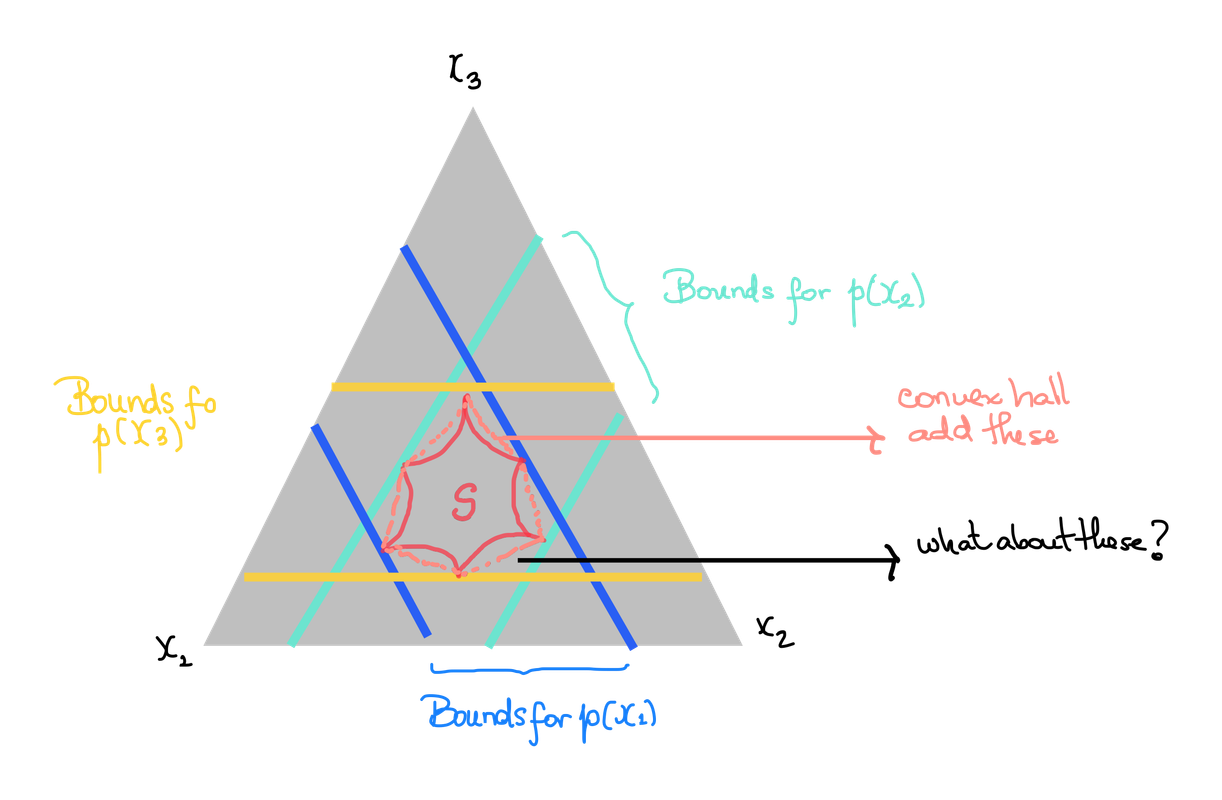
In order for Bob, in Example 1, to choose the most reasonable bet he should answer an important question: how should the bias of the coin be represented? One possible way of representing the bias of the coin is to consider, instead of just one probability measure, a set of probability measures, each of which corresponds to a specific bias, that is, we may consider the set $\mathcal{P}_C = \{\mu_\alpha \, : \, \alpha \in [0,1]\}$, where $\alpha$ denotes the bias of the coin. Now, we may handle uncertainty by defining the probabilities as follows: $\mu_\alpha(\{heads\}) = \alpha$ and $\mu_\alpha(\{tails\})= 1-\alpha$. This set of probabilities not only allows us to handle our ignorance about the bias of the coin, but also allows us to construct intervals to bound our ignorance. To construct such intervals we need to define what are called lower and upper probabilities. Specifically, if $\mathcal{P}$ is a set of probability measures defined over $2^{\Omega_C}$ where, $\Omega_C = \{head, tails\}$, and $U$ is an element of $2^{\Omega_C}$, we define the lower probability as

$$\mathcal{P}_*(U) = \inf \, \mathcal{P}(U),$$

and the upper probability as $$\mathcal{P}^*(U) = \sup \, \mathcal{P}(U).$$

The interval $[[\mathcal{P}_{\ast}(U), \mathcal{P}^{\ast}(U)]]$ is called estimate interval, since its length is a way of measuring the ambiguity or ignorance about the event $U$. For the case of the coin, we may see that the estimate intervals for the two possible outcomes, both have a length of 1, which tells us that there is maximal uncertainty about these events.

In spite of the names, upper and lower probabilities are not actually probabilities because they are not additive, instead lower probabilities are super-additive, and upper probabilities are sub-additive.However, in contrast with probability measures where the additivity property defines them, lower and upper probabilities are neither defined nor completely characterized by the super or sub-additivity property (the property that characterizes them is rather complex, those interested readers can refer to [1]. By allowing for a range of possible probability assignments, the approach of a set of probability measures allows uncertainty to be addressed. Moreover, lower and upper probabilities provide us with a way of bounding such uncertainty.

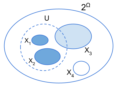
Inner and outer measures

As we already discussed, one of the problems of probabilities arises when the agent is not able to assign probabilities to all measurable sets. However, we may ask ourselves, what happens if we just ”remove” those measurable sets for which we do not have information? To illustrate these ideas, let’s use example 2. For this specific example, since we only have information about the numbers of red gummies, and the number of green and yellow gummies (togheter), we may consider the following sub-collection of events $\mathcal{S}_G= \{\{r\}, \{g,y\}, \{r,g,y\}, \emptyset\}.$. This sub-collection of events can be proven to be an algebra over $\Omega_G$. Moreover, this ”smaller” algebra is actually a subalgebra of the power set algebra $2^{\Omega_G}$ since $\mathcal{S}_G \subset 2^{\Omega_G}$. On this subalgebra we can define the measure $\mu_{{\mathcal{S}}_G}$ given by $\mu_{{\mathcal{S}}_G}(\{r\})=0.3$ and $\mu_{{\mathcal{S}}_G}(\{g,y\}) = 0.7$ which is well defined, it tells the same story illustrated in example 2, and it is consistent with Kolmogorov’s axioms. Since in this setting we have ”removed” those singletons sets corresponding to the yellow and green gummies, these events are undefined, and in principle, we cannot say anything about them. However, let’s define the following set of probability measures on the algebra $2^{\Omega_G}$, the set $\mathcal{P}_G = \{\mu_\beta : {\beta \in [0,0.7]}\}$ where, $\mu_\beta(\{r\}) = 0.3$, $\mu_\beta(\{g\}) = \beta$ and $\mu_\beta(\{y\}) = 0.7 - \beta$. One thing we may notice is that each measure $\mu_\beta \in \mathcal{P}_G$ is actually an extension of the measure $\mu_{{\mathcal{S}}_G}$, that is, for each $\beta$, the measures coincide on all sets of $\mathcal{S}_G$. Of course, if $U$ belongs to $2^{\Omega_G} \setminus \mathcal{S}_G$, then $\mu_{\mathcal{S}_G}(U)$ is not defined. But the extension of the measure is. That is, we may ask if it is possible to extend $\mu_{\mathcal{S}_G}$ to the whole algebra $2^{\Omega_G}$ so that we may have some information about those indefinite events that we want to studyt. Fortunately, this is indeed possible. Specifically, there are two canonical ways of extending $\mu_{\mathcal{S}_G}$ [3]. They are called inner and outer measures and they are defined, in general, as follows: let $\mathcal{S}$ a sub-algebra of $2^\Omega$ over a (finite) outcome space $\Omega$, $\mu_S$ a measure defined over the subalgebra and $U \in \mathcal{S}$. We define the inner measure induced by $\mu_S$ as

$${\mu_\mathcal{S}}_*(U) = \sup \bigl\{ \mu(V) \, : \, V \subseteq U, V \in \mathcal{S} \bigr\},$$

that is, as the largest measure of an $\mathcal{S}$-measurable set contained within $U$. On the other hand, the outer measure induced by $\mu_S$ is defined by

$${\mu_\mathcal{S}}^*(U) = \sup \bigl\{\mu(V) \, : \, V \supseteq U, \, V \in \mathcal{S} \bigr\},$$

that is, as the smallest measure of an $\mathcal{S}$-measurable set containing $U$. Therefore, in example 2 we have ${\mu_{{\mathcal{S}}G}}{\ast}(\{r\}) = {\mu_{{\mathcal{S}}G}}^{\ast}(\{r\}) = 0.3$, ${\mu{{\mathcal{S}}G}}{\ast}(\{y\}) = {\mu_{{\mathcal{S}}G}}{\ast}(\{g\}) = 0$, and ${\mu_{{\mathcal{S}}G}}^{\ast}(\{g\}) = {\mu{{\mathcal{S}}_G}}^{\ast}(\{y\}) = 0.7$. Here, again by means of the outer and inner measures, we may define interval estimates. If we define such intervals we have that the uncertainty in the event of choosing a red gummy is 0, while the uncertainty of the two other events will be 0.7. Just as with lower and upper probabilities, inner and outer measures are not probability measures: inner measures and outer measures are super-additive and sub-additive, respectively, instead of additive. By offering lower and upper bounds, inner and outer measures enable us to bound our ignorance. Moreover, they also allow us to ”deal” with those indefinite or non-measurable events that we leave out of our algebra from the very beginning, giving us information about them by considering the best possible approximations from within (inner) and from outside (outer).

Belief functions

As the examples given above have shown, additivity may be sometimes artificial. As we have seen, upper/lower probabilities and inner/outer measures, which are better at handling ignorance than probability measures, do not satisfy this requirement. Moreover, there exists a type of weighted function for which superadditivity (motivated above by Example 3) is actually part of its axiomatic definition. These functions are the so-called belief functions. They were introduced by Arthur P. Dempster in 1968 and expanded by Glenn Shafer in 1976. The Dempster-Shafer theory offers a powerful framework for representing epistemic uncertainty. Unlike classical probability theory, Dempster-Shafer theory allows for the representation of ignorance and partial belief, thus providing a more flexible approach to handling uncertainty.

A fundamental distinction between probability measures and Dempster-Shafer theory lies in their approach to additivity. While in classical probability, the Kolmogorov axioms enforce finite additivity, the Dempster-Shafer theory adopts finite superadditivity: $Bel(U \cup V) \geq Bel(U) + Bel(V), \text{ for } U \cap V = \emptyset$. This superadditivity allows Dempster-Shafer theory to capture uncertainty in a way that classical probability cannot. By not requiring strict additivity, this theory accommodates situations where the combined belief in two events can be greater than the sum of their individual beliefs, reflecting a more nuanced understanding of uncertainty.

To utilize Dempster-Shafer theory, we start with the concept of a frame of discernment, $\Omega$, which represents all possible outcomes in a given context (playing an analogous role as the sample space in probability theory). For example, in a football match between Argentina and Germany (Example 3 mentioned above), the frame of discernment would be: $\Omega = \{A, G, \text{Draw}\}$, where $A$ denotes “Argentina wins,” $G$ denotes “Germany wins,” and “Draw” represents a tie. Note that while $\Omega$ also denotes the sample space in probability theory, here it is used to define the frame of discernment.

The power set of $\Omega$, denoted $2^\Omega$, as previously explained when discussing probability theory, includes all subsets of $\Omega$, representing all possible events:

$2^\Omega = \{\emptyset, \{A\}, \{G\}, \{\text{Draw}\}, \{A, G\}, \{A, \text{Draw}\}, \{G, \text{Draw}\}, \{A, G, \text{Draw}\}\}$.

A mass function $m : 2^\Omega \rightarrow [0, 1]$ distributes belief across the elements of $2^\Omega$. This mass function must satisfy two key properties: $m(\emptyset) = 0$, which implies the empty set has zero belief, and $\sum_{X \in 2^\Omega} m(X) = 1$ which tells us that the total belief across all subsets of $\Omega$ sums to one.

This framework allows us to represent ambiguity and partial belief without requiring full certainty in any single outcome or in the entire frame. To illustrate this, let’s continue with the example of the football match between Argentina and Germany. Using classical probability, if we believe there is an equal likelihood for either team to win, we might assign: $\mu(A) = \mu(G) = 0.1 \Rightarrow \mu(A \cup G) = 0.2.$ In Dempster-Shafer theory, we can represent partial beliefs more flexibly. For instance: $Bel(A) = Bel(G) = 0.1,$ but given additional information suggesting a high likelihood that one team will win, we might have: $Bel(A \cup G) = 0.8.$ This reflects a stronger belief in the combined event without committing to either team individually.

In Dempster-Shafer theory, there are two key functions quantifying belief: the belief function $Bel$ and the plausibility function $Pl$. The belief function $Bel(U)$ sums the masses of all subsets $X$ contained within $U$ :

$$Bel(U) = \sum_{X \subseteq U} m(X).$$

The plausibility function $Pl(U)$ sums the masses of all subsets $X$ that intersect $U$:

$$Pl(U) = \sum_{X \cap U \neq \emptyset} m(X).$$

These functions provide lower and upper bounds on our belief in a hypothesis $U$.

Returning to our football match example, suppose we have the following Basic Belief Assignments: $m(\{A\}) = 0.1, m(\{G\}) = 0.1 , m(\{\text{Draw}\}) = 0.2$, and $m(\{A, G\}) = 0.6$.

We can then calculate the respective belief and plausibility functions as follows:

Belief Functions:

• $Bel(A) = 0.1$
• $Bel(G) = 0.1$
• $Bel(A \cup G) = 0.8$

Plausibility Functions:

• $Pl(A) = 0.7$
• $Pl(G) = 0.7$
• $Pl(\{\text{Draw}\}) = 0.2$

Notice that belief and plausibility functions are related by the following equation: $Pl(U) = 1 - Bel(\overline{U})$. This relationship shows that plausibility represents the extent to which we do not disbelieve U.

Finally, an essential feature of Dempster-Shafer theory is Dempster’s rule of combination, which allows for the integration of evidence from multiple sources. Given two independent bodies of evidence, represented by mass functions $m_1$ and $m_2$ over the same frame $\Omega$, the combined mass function is:

$$(m_1 \oplus m_2)(U) = \frac{1}{1-K} \sum_{U_1 \cap U_2 = U} m_1(U_1) m_2(U_2), \quad \forall U \neq \emptyset,$$

where, $K$ is the normalization factor representing the total conflict between $m_1$ and $m_2$:

$$K = \sum_{U_1 \cap U_2 = \emptyset} m_1(U_1) m_2(U_2).$$ Dempster’s rule ensures consistency by requiring that $K < 1$, meaning there is not total conflict between the two evidence sources.

As we have already seen one of the main differences between the measure theoretic approach and the approaches of imprecise probabilities discussed here is the relaxation of the additivity condition. However, it is worth saying that in other approaches of imprecise probability this condition is not even considered or is substituted for another one as happens in the case of possibility measures (see, for example, [1]). Each of the different approaches for handling uncertainty may be useful in different scenarios, and it will depend on the particular case we have to use one or another. The measure-theoretic probability is a well-understood framework and it has extensive support of technical results. However, as we stated here, this framework is by no means the only one and not necessarily the best one for every case-scenario. The set of probability measures extends the traditional probability approach by allowing for a range of possible probabilities, which is useful when there is uncertainty about the likelihoods themselves but, some information about the parameters “indexing” the probabilities is required. Belief functions, on the other hand, have proven themselves robustly effective in modelling and integrating evidence especially when combined with Dempster’s Rule of Combination [1]. Other approaches, which are not discussed in here, like partial preorders, possibility measures and ranking function may also be an interesting option to address uncertainty, in particular, for dealing with counterfactual reasoning [1].

Monads and imprecise probabilities

Recently, within the context of category theory numerous diagrammatic axioms have been proposed, facilitating the proof of diverse and interesting theorems and constructions in probability, statistics and information theory (see, for example, [4], [5], [6], [7], [8], [9], [10], [11], [12], [13], [14]). Because of this, a shift in the perspective of the foundational structure of probability theory has gained substantial momentum. In this new perspective a more synthetic approach to measure-theoretic probability is sought. The natural framework for this approach turns out to be that of a Markov category, that is, a symmetric monoidal category $(\mathsf{C},\otimes, I,s)$ in which every object is endowed with a commutative comonoid structure [9]. Since Markov categories have been serving as a fertile environment in providing new insights on probability theory it is natural to ask if these other approaches in handling uncertainty (lower/upper probabilities, inner/outer measures, belief functions, etc) may fit into this new synthetic perspective.

In some Markov categories the morphisms may be understood as ”transitions with randomness”, where this randomness may be “indentified” by means of the comonoid structure, that is, with this structure we may put a distinction between morphisms that involve randomness and those that do not [15]. Nevertheless, recent investigations show that their randomness may also be understood ”as the computational effect embodied by a commutative monad” [16]. More precisely, constructions of so-called representable Markov categories [12] can be understood as starting from a Cartesian monoidal category (with no randomness) and passing to the Kleisli category of a commutative monad that introduces morphisms with randomness. For example, in the category $\mathsf{Set}$ we may define the distribution monad $(\text{P}, \delta, \mu)$ where $\text{P}$ is the distribution functor assigning to each set $X$ the set of all finitely supported probability measures over $X$ and to each morphism $f: X \to Y$ the morphism $\text{P}f: \text{P}X \to \text{P}Y$ given by the pushforward measure. Here, the unit map $\delta_X: X \to \text{P}X$ is the natural embedding

$$\delta: X \to \text{P}X, \quad x \mapsto \delta_x,$$

where, $\delta_x: X \to [0,1], y \mapsto \delta_x(y)$ with $\delta_x(y) = 1$ for $x=y$ and $\delta_x(y) = 0$ otherwise, and the multiplication map is given by

$$\displaystyle \mu_X: \text{P}\text{P}X \to \text{P}X, \quad \pi \mapsto \mu_X(\pi),$$

which assigns to each measure $\pi$ over $PX$ the ”mixture” measure $\mu_X(\pi)$ over $X$ defined by $$\mu_X(\pi)(x) = \sum_{p \, \in \, \mathrm{P}X} \pi(p) p(x).$$

With this structure in mind, you may think about morphisms of the type $f: X \to \text{P}Y$. In the case of the distribution monad described above, to each $x \in X$, they assign a finitely supported probability measure $f_x$ over $Y$. These can be seen as morphisms with an uncertain output, or as some sort of generalized mapping allowing more ”general” outputs. We call these morphisms Kleisli morphisms [17]. For the particular case of the distribution monad, the Kleisli morphisms$f: X \to \text{P}Y$ where each $x$ is mapped to the probability distribution on Y, that is, to a function such that, $y \in Y \mapsto f(y|x)$, with $f(y|x)$ the components of a stochastic matrix. Moreover, the Kleisli category $\mathsf{Kl}(\mathrm{P})$, whose objects are those of $\mathsf{Set}$, and whose morphisms are the Kleisli morphisms can be endowed with a commutative comonoid structure. Furthermore, since we have $\text{P}I \cong I$, one can show that the Kleisli category $\mathsf{Kl}(\text{P})$ is a Markov category [12]. In fact, the category $\mathsf{FinStoch}$ is a full subcategory of it. Several Markov categories can be obtained in this way, for example $\mathsf{Stoch}$, is the Kleisli category of the Giry monad on $\mathsf{Meas}$ (see [12] and the other examples in there).

An intriguing question then emerges from the topics discussed herein: Is there a commutative monad $(\mathcal{I},\eta,\mu)$ over some suitable category such that the morphisms of its Kleisli category $\mathsf{Kl}(\mathcal{I})$ model a certain type of imprecise probability? Or in other words, do imprecise probabilities (upper and lower probabilities, inner and outer measures, belief functions, etc) form Markov categories? This possible interesting byproduct between imprecise probabilities and category theory has already captured the attention of members of the communities of Probability and Statistics and Category Theory. Moreover, quite recently Liell-Cock and Staton have tried to address a similar question in [18]. Tobias Fritz and Pedro Terán have also studied a similar question involving possibility measures in an unpublished work. We hope very soon that a plethora of works is dedicated to studying such interesting byproduct.

References

1. Joseph Y. Halpern. (2017). Reasoning about uncertainty. The MIT Press.

2. Edwin T. Jaynes. (2003). Probability Theory. The Logic of Science. Cambdridge University Press.

3. Marshall Evans Munroe. (1953). Introduction to MEASURE AND INTEGRATION. Cambridge, Mass., Addison-Wesley.

4. Michèle Giry (1982).A categorical approach to probability theory. In: Banaschewski, B. (eds) Categorical Aspects of Topology and Analysis. Lecture Notes in Mathematics, Volume 915. Springer, Berlin, Heidelberg. DOI: 10.1007/BFb0092872

5. Prakash Panangaden (1999). The Category of Markov Kernels. Electronic Notes in Theoretical Computer Science, Volume 22. DOI: 10.1016/S1571-0661(05)80602-4

6. Peter Golubtsov (2002). Monoidal Kleisli Category as a Background for Information Transformers Theory. Processing 2, Number 1.

7. Jared Culbertson and Kirk Sturtz (2014). Postulates for General Quantum Mechanics. Appl Categor Struct, Volume 22. DOI: 10.1007/s10485-013-9324-

8. Tobias Fritz, Eigil Fjeldgren Rischel (2020). Infinite products and zero-one laws in categorical probability. Compositionality, Volume 2. DOI: 10.32408/compositionality-2-3

9. Tobias Fritz (2020). A synthetic approach to Markov kernels, conditional independence and theorems on sufficient statistics. Advances in Mathematics, Volume 370. DOI: 10.1016/j.aim.2020.107239

10. Bart Jacobs and Sam Staton (2020). De Finetti’s Construction as a Categorical Limit. In: Petrişan, D., Rot, J. (eds) Coalgebraic Methods in Computer Science. CMCS 2020. Lecture Notes in Computer Science(), vol 12094. Springer, Cham. DOI: 10.1007/978-3-030-57201-3_6

11. Tobias Fritz,Tomás Gonda and Paolo Perrone (2021). De Finetti’s theorem in categorical probability. Journal of Stochastic Analysis, Volume 2. DOI: 10.31390/josa.2.4.06

12. Tobias Fritz, Tomás Gonda, Paolo Perrone and Eigil Fjeldgren Rischel (2023). Representable Markov categories and comparison of statistical experiments in categorical probability. Theoretical Computer Science, Volume 961. DOI: 10.1016/j.aim.2020.107239

13. Tobias Fritz and Andreas Klingler (2023). The d-separation criterion in Categorical Probability. Journal of Machine Learning, Volume 24. DOI: 22-0916/22-0916

14. Sean Moss and Paolo Perrone (2023). A category-theoretic proof of the ergodic decomposition theorem. Ergodic Theory and Dynamical Systems, Volume 43. DOI: 10.1017/etds.2023.6

15. Paolo Perrone (2024). Markov Categories and Entropy. IEEE Transactions on Information Theory, Volume 70. DOI: 10.1109/TIT.2023.3328825.

16. Sean Moss and Paolo Perrone (2022). Probability monads with submonads of deterministic states. In: Proceedings of the 37th Annual ACM/IEEE Symposium on Logic in Computer Science. Association for Computing Machinery, LICS ‘22. DOI: 10.1145/3531130.3533355.

17. Paolo Perrone (2024). Starting Category Theory. World Scientific Book.

18. Jack Liell-Cock, Sam Staton (2024). Compositional imprecise probability. arXiv: 2405.09391.