Outline of this blog

Throughout this blog post, we will present many of the ideas in the paper “String Diagrams for lambda calculi and Functional Computation” by Dan R. Ghica and Fabio Zanasi from 2023. In the first section, we will recall the untyped lambda and simply typed lambda calculus. In the next section, we will review the basic concepts and notation of string diagrams for monoidal categories. Then, we will extend our graphical language with the necessary notation to represent terms in a Cartesian Closed Category. Finally, in the last section, we will present the operational semantics for lambda calculus based on string diagrams and study a case example of arithmetics operations and recursion.

Lambda calculus quick quick crash course

We will start by reviewing one of the first and more “simple” models of computation: The lambda calculus. The lambda calculus was originally developed by Alonzo Church when he was studying problems on the foundations of mathematics. Alan Turing proposed almost simultaneously its famous model of computation based on an abstract machine that moves along an infinite tape. The lambda calculus is equivalent to Turing’s model. If we would like to have an intuition about the difference between the two models we would say that the lambda calculus is closer to the idea of software while Turing machines are closer to hardware. The lambda calculus has had a huge influence and applications to different areas of Computer science, logic, and mathematics. In particular to functional programming languages, as lambda calculus provides the foundational theoretical framework upon which functional programming languages are built.

Lambda-calculus is based on a rewrite system. Every term in lambda calculus is morally a function, you can apply functions and abstract functions.

More precisely, a lambda term is defined inductively as follows:

• A variable $x,y,z, \cdots$ is a lambda term;
• Given two lambda terms $f$ and $x$, $(fx)$ is a lambda term representing the application of $f$ to $x$;
• Given a variable $x$ and a lambda term $t$, $(\lambda x. t)$ is a lambda term representing the function taking an $x$ as input and returning $t$ where $x$ is a bound variable in $t$, this is called an abstraction.

Function application is left-associative by convention.

Three reductions are usually defined on lambda terms, $\alpha$-conversion allows to change bound variables names to avoid naming conflicts, $\beta$-reduction apply a function to its argument by replacing the bound variable with the argument, and $\eta$-reduction which identifies two functions if they give the same output for every input.

We will focus on $\beta$-reduction as we don’t aim for a super formal approach, and $\alpha$-conversion can be avoided in different ways (using De Bruijn index notation, for instance). $\beta$-reduction is confluent when working up to $\alpha$-conversion, so that is what we are going to assume throughout this blog.

How to represent simple data types in untyped lambda calculus? Since in untyped lambda calculus everything is a function, the idea is to encode simple data types using only functions in a consistent way. For instance, we can define booleans in the following manner: $True$ := $(\lambda x. \lambda y. x)$ and $False$ := $(\lambda x. \lambda y. y)$.

The idea is that a boolean is meant to be used in a if-then-else statement, let $T$ be the ‘then’ expression and $E$ be the ‘else’ expression, the if-then-else statement can be expressed with $BTE$ where $B$ is a boolean. Indeed, if $B = True$ then we have $TrueTE$ which is equal by definition to $(\lambda x. \lambda y. x)TE$ which reduces to $T$. If $B = False$, then $FalseTE = (\lambda x. \lambda y. y)TE$ yields $E$ after two $\beta$-reduction.

Logical connectors ‘and’, ‘or’, ‘implies’, ‘not’, can be implemented using if-then-else statements, for example $and := (\lambda B1. \lambda B2. B1 B2 False)$ which reads if $B1$ is true then return $B2$ else return $False$.

We can also represent natural numbers by successive application of a function, these are the Church numerals:

• 0 := $(\lambda f. \lambda x. x)$ a function which applies $f$ 0 time;
• 1 := $(\lambda f. \lambda x. f x)$ a function which applies $f$ 1 time;
• 2 := $(\lambda f. \lambda x. f (f x))$ a function which applies $f$ 2 times;
• $n+1$ := $(\lambda f. \lambda x. f (n f x))$ recursively, the successor of a number $n$ applies $f$ one more time to $x$ than $n$.

We can define usual functions on numbers:

• $succ$ := $(\lambda n.(\lambda f. \lambda x. f (n f x)))$
• + := $(\lambda n. \lambda m. \lambda f. \lambda x. m f (n f x))$
• * := $(\lambda n. \lambda m. \lambda f. \lambda x. m (n f) x)$ and so on

What we described above is untyped lambda calculus, but it lacks certain properties due to its computability power. For example, it allows paradoxes such as Kleene-Rosser paradox and Curry’s paradox. To have a better rewriting system, Alonzo Church introduced simply typed lambda calculus.

The idea is to give a type to variables to prevent self application of function. To this end, we consider a typing environment $\Gamma$ and typing rules:

• $\frac{x:t \in \Gamma}{\Gamma \vdash x : t}$ This means that a typing assumption in the typing environment should be in the typing relation;

• $\frac{\text{c is a constant of type t}}{\Gamma \vdash c : t}$ This means that terms constant have appropriate base types (e.g. 5 is an integer);

• $\frac{\Gamma, x:t_1 \vdash y:t_2}{\Gamma \vdash (\lambda x:t_1 . y) : (t_1 \to t_2)}$ This means that if $y$ is of type $t_2$ when $x$ is of type $t_1$, then the $\lambda$ abstraction $(\lambda x:t_1. y)$ is of the function type $(t_1 \to t_2)$;

• $\frac{\Gamma \vdash x : t_1 \to t_2 \quad \Gamma \vdash y : t_1}{\Gamma \vdash (xy) : t_2}$ This means that when you apply a function of type $t_1 \to t_2$ to an argument of type $t_1$ it gives a result of type $t_2$.

When writing $\lambda$ terms, we now have to specify the type of the variables we introduce. The examples above now become:

• 0 := $(\lambda f : t \to t. \lambda x : t. x)$
• 1 := $(\lambda f : t \to t . \lambda x : t. f x$
• 2 := $(\lambda f : t \to t . \lambda x : t. f (f x)$
• $succ$:= $(\lambda n : (t \to t) \to (t \to t) .(\lambda f : t \to t . \lambda x : t. f (n f x)))$
• + := $(\lambda (t \to t) \to (t \to t). \lambda (t \to t) \to (t \to t). \lambda f : t \to t. \lambda x : t. m f (n f x))$
• * := $(\lambda n : (t \to t) \to (t \to t). \lambda m : (t \to t) \to (t \to t). \lambda f : t \to t. \lambda x : t. m (n f) x)$

Crucially, we can no longer apply a function to itself: let’s suppose $x$ has type $t_1$, then $xx$ would mean that $x$ must be a function taking $t_1$ as an argument, so $t_1 \to t_2$, but it now means that $x$ should take an argument of type $t_1 \to t_2$ so $x$ would be of type $(t_1 \to t_2) \to t_3$ and so on which is impossible.

Because we can no longer apply a function to itself, simply typed $\lambda$ calculus is no longer Turing complete and every program eventually halts. It is therefore less powerful but has nicer properties than untyped $\lambda$ calculus. From now on, we will work with simply typed $\lambda$ calculus not just because of its rewrite properties but also because of its strong connections with category theory.

Everything we have explained in a very hurried and informal manner in this section, can be fully formalized and treated with mathematical rigor. The objective of this section is to ensure that those not familiar with lambda calculus do not find it an impediment to continue reading. If the reader wishes to delve deeper or see a more formal treatment of what has been explained and defined in this section, they can refer to “Lambda calculus and combinator: an introduction” by Hindley and Seldin for a classical and treatment or to “Introduction to Higher order categorical logic” by Lambek and Scott for a more categorical approach.

String diagrams

String diagrams for monoidal categories

Why use symmetric monoidal categories? Monoidal categories arise all the time in mathematics and are one of the most studied structures in category theory. In the more applied context, a monoidal category is a suitable algebraic structure if we want to express processes with multiple inputs and multiple outputs.

String diagrams are nice representations of terms in a symmetric monoidal category which exploits our visual pattern recognition of a multigraph’s topology to our advantage.

As a quick reminder, a monoidal category is a sextuplet $(\mathcal{C}, \otimes : \mathcal{C} \times \mathcal{C} \to \mathcal{C}, I, \alpha : (- \otimes -) \otimes - \implies - \otimes (- \otimes -), \lambda : (I \otimes -) \implies -, \rho : (- \otimes I) \implies -)$ where:

• $\mathcal{C}$ is a category;
• $\otimes$ is a bifunctor called a tensor product;
• $I$ an object called the unit;
• $\alpha$ is a natural isomorphism called the associator;
• $\lambda, \rho$ are natural isomorphisms called respectively the left and right unitor;

such that the triangle and the pentagon diagrams commute:

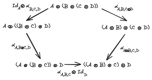
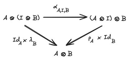
A strict monoidal category is a monoidal category where the associator and the unitors are identities, every monoidal category is equivalent to a strict one so we may use strict monoidal categories from now on.

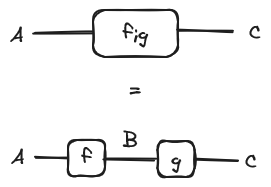
With string diagrams, the objects of the category are represented as labelled wires, the morphisms as named boxes and the composition of two morphisms is the horizontal concatenation of string diagrams and the tensor product of two objects/morphisms the vertical juxtaposition:

We already see the usefulness of string diagrams when seeing the interchange law. The interchange law states that $(\forall f,g,h,i \in Ar(\mathcal{C}))\quad (f;g) \otimes (h;i) = (f \otimes h) ; (g \otimes i)$.

It becomes trivial when seen as a string diagram:

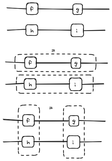
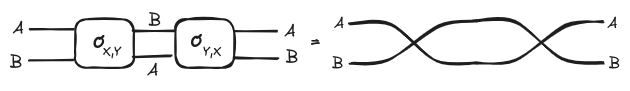
A symmetric monoidal category is a monoidal category equipped with a natural isomorphism $\sigma$ called a braiding such that $\sigma_{A,B} ; \sigma_{B,A} = Id_{A \otimes B}$. We will represent the braiding morphisms are as follows:

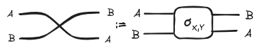
Again the topology of the string diagram’s underlying multigraph reflects the properties of the braiding when the monoidal category is symmetric.

To put it in a nutshell, string diagrams are great visualization tools to represent morphisms in a symmetric monoidal category because they exploit our visual pattern recognition of the topology of a graph: we intuitively understand how wiring boxes work.

Functors boxes

So far, we have reviewed the standard notation for string diagrams on monoidal categories. Now we will introduce how to represent functors in our graphical language.

Let $\mathcal{C}$ and $\mathcal{D}$ be two categories. And let $F: \mathcal{C} \to \mathcal{D}$ be a functor between them. Then the functor F applied to a morphism f is represented as an F-labelled box:

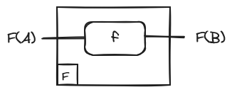
Intuitively, the box acts as a kind of boundary. What it is inside the functor box (wires and boxes) lives in $\mathcal{C}$, while the outside lives in $\mathcal{D}$.

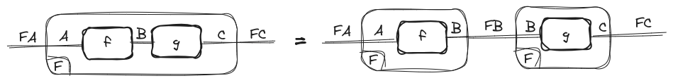
As an example, the composition law of functors would look like this using the above notation:

Adjoint and abstraction

One of the categorical constructions we will use the most throughout this blog is adjunctions, so we would like to represent them in our graphical notation. In particular, we will make use of the unit/counit definition. The reason for doing this, is, first because the unit and counit of the particular adjunction pair that we are interested in will play an important role, and second because the unit/counit presentation is arguably the best when using string diagrams.

What should we add to represent adjunctions in our graphical notation? Well… nothing! We already have a notation for functors. Natural transformations, from the point of view of string diagrams, are just collections of morphisms, so the components of a natural transformation are represented as boxes, just like any other morphism in the category. However, since the unit and counit will play a fundamental role, it will be convenient for us to have a special notation for both.

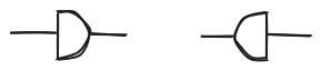
We will represent the unit as a right-pointing half-circle with the object components in the middle. For the counit, it is analogous but points to the left.

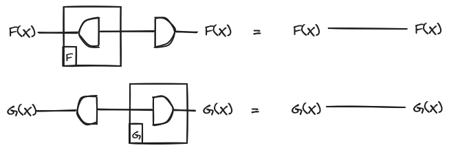
Now the equations look like this:

The particular pair of adjoints that we are interested in is the pair consisting of the tensor product functor $F_X (A) = A \otimes X:\mathcal{C} \to \mathcal{C}$ and its right adjoint $G_X(A)$ which we write as $X \multimap A$, where $\mathcal{C}$ is a monoidal category. This adjunction is also usually written as $- \otimes X \vdash X \multimap -$

When the functor $- \otimes B : \mathcal{C} \to \mathcal{C}$ has a right adjoint $B \multimap - : \mathcal{C} \to \mathcal{C}$ we say that $\mathcal{C}$ is a closed monoidal category.

The importance of this pair of adjoints lies in their counit and unit, which allow us to represent the idea of application and abstraction, that one we presented in the previous section, respectively.

The first one makes total sense because if we analyze the form of the counit, we will discover that it perfectly matches the function application form: $$\epsilon_A: F( G A) \to A$$

$$\epsilon_A: (X \multimap A) \otimes X \to A$$

On the other hand, the counit has the following form:

$$\eta_A : A \to G (F A)$$

$$\eta_A : A \to X \multimap (A \otimes X)$$

If we mix the counit with the $X \multimap -$ functor we can do abstraction of morphisms and currying (note that abstraction is currying with the unit: $(I \otimes A \to B) \mapsto (I \to (A \multimap B))$). So for any morphism $f: X \otimes A \to Y$ we will denote its abstraction as $\Lambda_X(f): A \to X \multimap Y$

We will use this construction a lot so we will use a syntactic sugar to denote it in our graphical formalism.

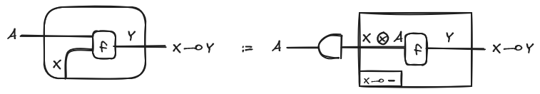
Notice that this syntactic sugar is quite suggestive since the hanging wire gives us the idea of a quantified variable waiting to be used, but it is important to note that this is just a graphical convention.

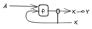
Another usual notation is the clasp of the Rosetta Stone paper by Baez and Stay:

Now Cartesian

We finish this section with the last ingredient necessary to represent graphically the terms of a Cartesian Closed Category, which is the product object. The motivation for having this construction is that, in our simple programming language, we would like to be able to represent functions that take more than one parameter. Similarly, it would be useful to have the ability to duplicate the output of a function or discard it (yes, this is no quantum computing!), which is directly related to the previous point.

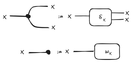
With this in mind, we introduce two natural transformations $\delta_A: A \to A \otimes A$ and $\omega_A: A \to I$, which we call copy and delete, respectively. Before giving the equations necessary to call a category $\mathcal{C}$ “cartesian”, as we mentioned before, these natural transformations represent the ideas of duplicating and discarding the output of a function.

Since these two constructions will play a fundamental role in our task of representing functional programs, we will give them a special syntax:

And as we ask them to be natural, the naturality condition looks like this:

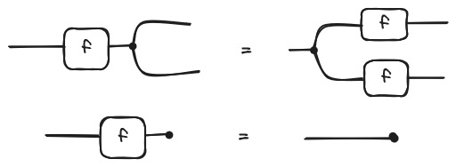
So finally, we will say that a symmetric monoidal tensor is a Cartesian product if, for each object $A$ in the category, the above-mentioned monoidal transformations $\delta_A$ and $\omega_A$ exist such that:

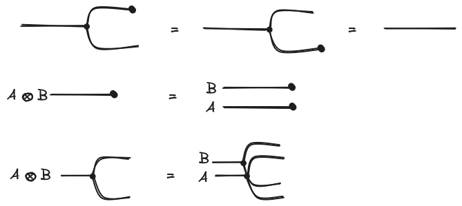
Note how we are expressing the properties directly using string diagrams! Just in case you’d like to see how these properties look in classical notation, here they are:

$$\omega_{A \otimes B} =\omega_A \otimes \omega_B$$

$$\delta_{A \otimes B} = \delta_A \otimes \delta_B; id_A \otimes \sigma_{A,B} \otimes id_B$$

$$\delta; id \otimes \omega = \delta; \omega \otimes id = id$$

A fun exercise for the non-lazy reader: This product definition is not the standard in category theory literature, which tends to use universality. How would you prove the equivalence between the two definitions using string diagrams? (for a solution see definition 3.13, chapter 3 of “String Diagrams for lambda calculi and Functional Computation” by Dan R. Ghica and Fabio Zanasi)

Some examples

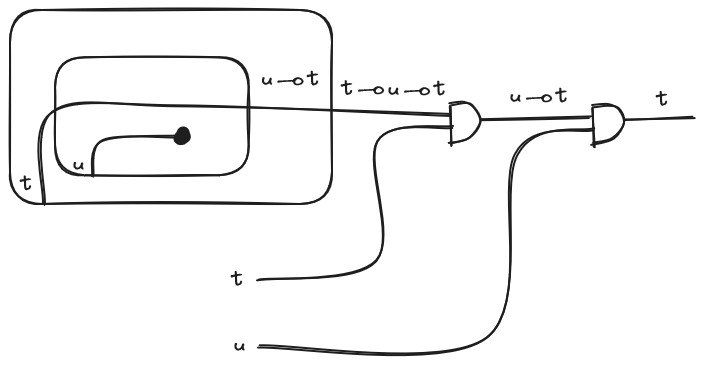
Now that we have all the necessary structure, let’s look at some examples of diagrams representing terms in the lambda calculus. Let’s start with the identity applied to itself $(\lambda x.x)(\lambda y.y)$. We have two abstractions and one application. Its string diagram representation is:

Now let’s draw the $True$ function defined earlier which is: $(\lambda x : t. \lambda y : u. x)$. This one consists of only two abstractions:

And if we would like to apply the previous function:

A comment on the relationship between lambda calculus

Although in the previous examples, we have been using it implicitly, we never provided the explicit relationship between lambda calculus and its respective category. For the sake of completeness and as a technical aside, we briefly comment that to construct the categorical interpretation, we take the types as objects of the category, and the morphisms are given by the tuples $(x, t)$ where $x: X$ is a variable and $t: Y$ is a term with the only possible free variable is x. And the composition is giving by chaining function applications, i.e. we take the output of one function and use it as the input for another (This can be formalized through term substitution). It is not the goal of this blog to provide a formal treatment of this (although it is a very interesting topic for a blog!). Interested readers can refer to the famous text “Introduction to Higher Order Categorical Logic” by Lambek and Scott.

The operational semantics

Now we have all the prerequisites for presenting our main topic. We are going to give an operational semantics based on string diagrams. This will consist of a series of rules that allow us to represent computation as a sequence of applications of such rules. But before doing that we have to decide a little detail, we must establish our evaluation strategy. When computing the application $fx$ you could first evaluate the argument $x$ and then apply $f$ to $x$ (call-by-value strategy) or you could first substitute $x$ in the body of $f$ and postpone the evaluation of $x$ (call-by-name strategy). For this blog, we will use the call-by-value strategy.

Now we can start to describe our operational semantics. First we will add a decorator to the string diagrams. This decorator is a syntactic construct applied to a specific wire, used for redex search and evaluation scheduling. Our interpretation of the decorator is as follows: when the decorator points left, it indicates the part of the string diagram that is about to be evaluated. When the decorator points right, it signifies that the indicated part has just been evaluated. With this in mind, the rules that will model the behavior of the decorator, and therefore execution, are the following ones:

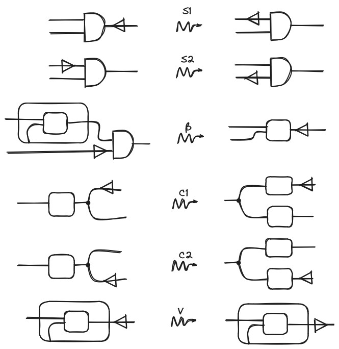
We argue that most of the rules are quite intuitive after some contemplation but let’s explain them a little:

• The first two (S1 and S2) models what we just said before about the evaluation strategy: (S1) For evaluating an application first we evaluate the function and (S2) After evaluating a function, evaluate the argument.
• This rule represents the $\beta$ rule of lambda calculus and says that after evaluating the argument, evaluate the result.
• The next two are about how to treat copying: (C1) When encountering a copying node, copy in both branches of the boxes, and (C2) is analogous but from the other side.
• The last one says that the abstraction is a value, here we won’t get into detail about this but basically, this means that when we encounter a lonely abstraction we stop the evaluation (note the change of direction of the decorator).

A parenthesis about rewriting: The reader might have noticed that we are talking about “rewriting” string diagrams, but at no point do we formally define what this means or how we can do it. This is beyond the scope of this blog, but for the curious reader, we strongly recommend our colleagues’ blog on the mathematical foundation behind string diagram rewriting:

Before we start adding cool stuff to our simply-type lambda calculus let’s see our first basic example. Let’s apply our operational rules to the string diagram of the identity function that we showed in the previous section:

Aritmetic, logic operations, and recursion

Let’s have a little fun and start defining the operations we would like to have in our language. We will provide the definitions of these operations and their operational semantics.

First, for doing arithmetics, we start adding a numerical type $Num$, with its respective constants that will have the form $m,n,...: I \to Num$. Let’s add a binary arithmetic operator. Now we need to think about what rewrite rules we are going to add. It is not hard to come up with the following rules:

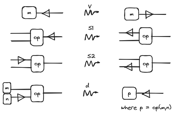
The first three are “reused” as they come from the order of evaluation and the idea that the constants are values and require no further evaluation. And finally, we have a reduction rule that tells us how to apply the operator to two constants. For example, for the operator $+$, there would be a rule for every pair of integers $(m,n)$ (e.g. $1+1=2$, $1+2=3$, and so on).

Note that those rules work for any binary operation by simply changing rule $d$!

Our last example consists of one of the most common characteristics in all modern programming language: Recursion. As with the previous example first we need to introduce a recursion operation, which we call $rec$, with the following rule: $$rec(\lambda f.u) = u[f/rec(\lambda f.u)]$$

The right side of the rule is just a fancy way of saying “the term that we get replacing f for every occurrence of $\lambda f. u$ in u”. Note how this rule doesn’t reduce the original term but expands it!

Then the structural rule that we will add for the above operation is the following one:

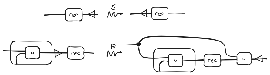
Why do these rules work? Well, the first one is obvious; it is just the analog of the structural rules but for unary operations. However, the second rule is trickier than the previous ones we have presented. This rule, whenever it encounters an abstraction already executed with the $rec$ operation following it, uncurry the $u$ function and passes the same diagram as second argument before the rewriting. It is important to note that this rule does not contract the diagram but expands it.

If we start repeatedly applying this rule, we get something like this:

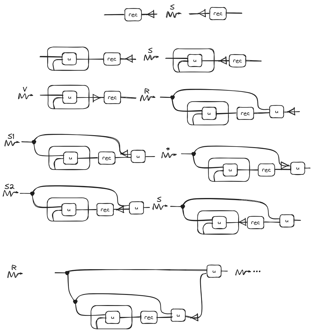
Of course, if we want to have a finite diagram, we should provide an $u$ that includes a base case, ensuring that the expansion stops at some point.

Another fun exercise for the non-lazy reader: How could we add an if-then-else operation to our language?

Hint: we should first introduce have a new type $Bool$ (with it respective two constants) and then an operation with the following type: $Bool \times Num \times Num \to Num$. Now what remains is to provide the definition of the operation and the operational rules for the string diagram interpretation.

Conclusion

Throughout the blog, we not only reviewed the notation of string diagrams for monoidal categories, but also explored how to represent the entire categorical structure behind simply typed lambda calculus. With this in hand, we developed a set of intuitive rules for modeling computation, in the style of operational semantics, which allowed us to add the desired features to our basic language. In particular, we provided examples of operations and recursion, but it doesn’t stop there, we invite the readers to have fun with what they’ve learned and see what features of their favorite programming language they can represent with this model. On the other hand, this blog can be considered another great example of the power of string diagrams. In particular, we, the authors, see it as a significant motivation for our research topic during the research week previous to the ACT conference in Oxford, which will focus on algorithmic methods behind certain rewriting problems of the kind of string diagrams presented in this blog.