An Invitation to Geometric Higher Categories
Posted by David Corfield
.")
Guest post by Christoph Dorn
While the term “geometric higher category” is new, its underlying idea is not: coherences in higher structures can be derived from (stratified) manifold topology. This idea is central to the cobordism hypothesis (and to the relation of manifold singularities and dualizability structures as previously discussed on the -Category Café), as well as to many other parts of modern Quantum Topology. So far, however, this close relation of manifold theory and higher category theory hasn’t been fully worked out. Geometric higher category theory aims to change that, and this blog post will sketch some of the central ideas of how it does so. A slightly more comprehensive (but blog-length-exceeding) version of this introduction to geometric higher categories can be found here:
Today, I only want to focus on two basic questions about geometric higher categories: namely, what is the idea behind the connection of geometry and higher category theory? And, what are the first ingredients needed in formalizing this connection?
What is geometric about geometric higher categories?
I would like to argue that there is a useful categorization of models of higher structures into three categories. But, I will only give one good example for my argument. The absence of other examples, however, can be taken as a problem that needs to be addressed, and as one of the motivations for studying geometric higher categories! The three categories of models that I want to consider are “geometric”, “topological” and “combinatorial” models of higher structures. Really, depending on your taste, different adjectives could have been chosen for these categories: for instance, in place of “combinatorial”, maybe you find that the adjectives “categorical” or “algebraic” are more applicable for what is to follow; and in place of “geometric”, maybe saying “manifold-stratified” would have been more descriptive.
But let’s get to the promised example of how these three categories of models work and how they relate. We start with the archetypical model of a type of higher structure: namely, with topological spaces. Unsurprisingly, topological spaces fall firmly into the category of topological models. The type of higher structure modelled by topological spaces deserves a name: we will refer to them as homotopy types. There is a second well-known model for homotopy types, namely, -groupoids. Unlike spaces, whose theory is based on the continuum , -groupoids are discrete structures whose data is captured by collections of morphisms in each dimension . This makes -groupoids a prime example of a ‘combinatorial’ (or, ‘algebraic’, or, ‘categorical’) model of a higher structure. (I should point out that I am being vague about concrete definitions of the above named ‘models’; for instance, ‘spaces’ could be, more concretely, taken to mean CW complexes, and -groupoids could be taken to mean Kan complexes.) Despite being rather different in flavour, the higher theory (i.e. the homotopy theory) of topological spaces and the higher theory of -groupoids turn out to be equivalent. The two models are related by two important constructions: we can pass from spaces to -groupoids by taking the fundamental categories of spaces (usually referred to as their ‘fundamental -groupoids’), and, conversely, we can realize -groupoids as spaces.
Now the interesting question: what is the geometric counterpart to the above topological and combinatorial models? In different words, how can we understand the homotopy theory of spaces in terms of a theory of manifold-stratified structures? The answer is given by the theory of cobordisms, or more precisely, stratified cobordisms. The most well-known instance of how cobordisms and spaces relate in this sense is the classical Pontryagin theorem. The theorem describes the isomorphism
between the cobordism group of smooth (normal) framed -manifolds in and the th homotopy group of the -sphere. The resulting relation between smooth manifold theory and homotopy theory is incredibly ubiquitous in modern Algebraic Topology (and, relatedly, in Physics) but often implicitly so — in the words of Mike Hopkins, Pontryagin’s theorem itself marks the point in time at which Algebraic Topology became ‘modern’.
Importantly for us, the theorem generalizes from spheres to arbitrary spaces (or, more precisely, CW complexes): namely, the th homotopy group of any space can be understood in terms of the framed stratified cobordisms group of framed -stratifications of (where, roughly, an ‘-stratification’ is a stratification whose singularity types are determined by the ‘dual cells’ of ). Formulaically, this may be expressed by writing
The details of this generalization are spelled out in [1, Ch. VII], in a chapter titled “the geometry of CW complexes”, but really the basic idea of the construction remains essentially the same (for the experts: instead of working with a regular value point of , we work with a regular dual stratification of the CW complex ). To summarize, we can study the homotopy groups of spaces, or, in combinatorial terms, the higher morphisms in -groupoids, by means of framed stratified cobordisms. The relation between the geometry of stratified cobordisms and the homotopy theory of spaces can be conceptually thought of as a process of dualization (which translates stratification data back into cells, and we will return to this later on).
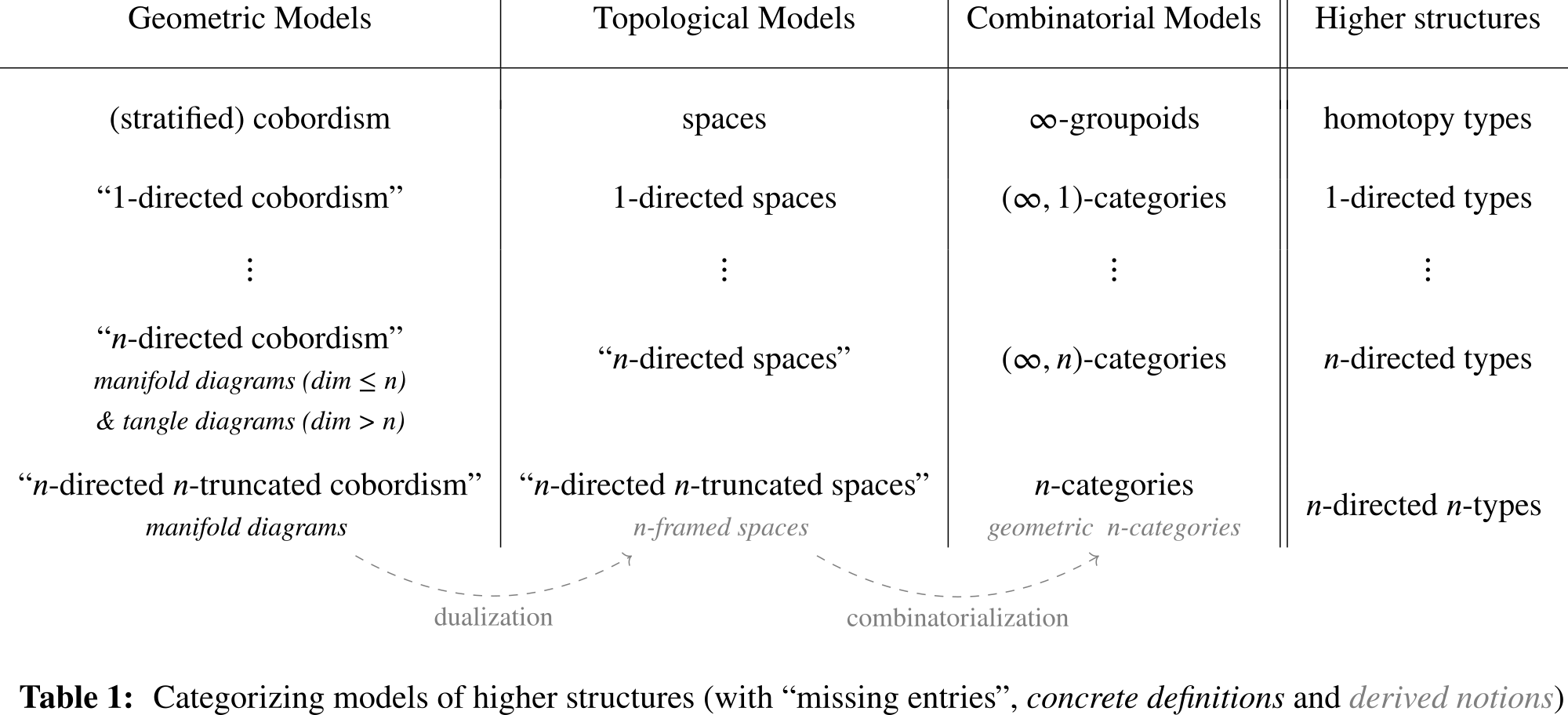
The main point I now want to make is that the trilogy of geometric, topological, and combinatorial models exemplified above in the case of homotopy types should also extend to other types of higher structures. In particular, -categories and -categories should admit both topological models and geometric models — however, these classes of models haven’t been much explored so far (as an aside, in the -case there is the theory of -spaces which appears to be an existing topological counterpart to -categories even though I’m unsure how much this relation has been formally explored). The situation is summarized in Table 1 below, in which we have filled in precisely some of the missing entries for geometric and topological models of higher structures: to indicate their conceptual nature, names of these models have been kept in quotes.
At a first glance, it seems like finding concrete definitions for these directed geometric models would be a tall order. After all, the theory of stratified cobordisms itself has its mathematical depths, and realizing the step from -groupoids (say, Kan complexes) to concrete definitions of -categories is not necessarily an obvious one.
But this is where things may get exciting. Indeed, by the end of this blog post I hope to have convinced you that the geometric models of higher structures may, in fact, get much easier when passing to the directed setting of -categories. Moreover, to then study the undirected setting (i.e., in combinatorial terms, the case of higher categories with invertible morphisms) from the perspective of directed geometric models provides a refined view on the computational intricacies of invertibility.
Of course, in order to be able to tell this story, I will have to shortly show you some concrete notions that aim to realize the geometric models outlined above. The notions go by the names of manifold diagrams resp. tangle diagrams, the latter being the relevant notion when considering invertible morphisms. Both notions have been added to Table 1 in their respective places (note that the -case requires us to deal with manifold diagrams in and below dimension , and with tangle diagrams above dimension ). Neither of these notions should come as a complete surprise, as we are already familiar with some of their instances: manifold diagrams specialize to string diagrams in dimension , i.e. they generalize the latter notion to arbitrary higher dimensions; and, (unstratified, framed) tangle diagrams formalize in all dimensions the pictures you are likely to draw when thinking about the tangle hypothesis!
Importantly, note that I wrote that the notions ‘aim to realize’ the aforementioned geometric models. Indeed, how do we measure ‘correctness’ of our definitions of manifold diagrams? Unfortunately, no reasonably-straight-forward benchmark for models of directed geometry exists at this point (actually, the same was in some sense true for manifolds when they were discovered, but they were quickly accepted due to their ubiquity in mathematics and physics). Certainly, passing from geometry to combinatorics in Table 1, a comparison to existing models of -categories would provide such a benchmark, but work remains to be done towards developing this relation, including the development of a more comprehensive theory of geometric higher categories (we will briefly discuss the case of ‘free’ geometric higher categories later). Today, I want to focus mainly on directed geometric models in the left column in Table 1. Indeed, I argue that these geometric models may very much deserve your interest on their own for the following ‘more elementary’ reasons.
Simplicity and ubiquity. Firstly, the definitions of manifold and tangle diagrams are simultaneously simple and expressive: both definitions succeed in encompassing large classes of known examples, including ordinary string diagrams and surface diagrams, knot and surface-knot diagrams, as well as their respective moves (Reidemeister moves and ‘movie moves’), and smooth manifold singularities such as Arnold’s ADE singularities [2].
Trilogy of models. Secondly, and this is a central part of the story, the theory of manifold and tangle diagrams comprises powerful dualization and combinatorialization results. From these results, one may then try to derive natural translations between all three columns of Table 1: in the topological column this leads to notions of directed spaces which we refer to as framed spaces; in the combinatorial column we obtain notions of higher categories which we refer to as geometric higher categories. (Note, both terms are used in a broad sense here, with concrete details of their respective theories being the topic of ongoing research). In the resulting combinatorial models, higher-categorical coherences are naturally related to stratified manifold isotopies!
Application. Thirdly and lastly, even without higher structures as our primary object of study, manifold and tangle diagrams provide a new tool at the interface of combinatorial higher algebra and differential topology. This leads to interesting questions such as the precise nature of the relation between diagram combinatorics and differential singularities (which I will briefly return to later), and a potentially ‘natural’ approach to combinatorial encodings of smooth structures.
Now that we have a rough idea about what makes geometric models of higher structures ‘geometric’, and why they might be interesting, let’s see some definitions!
From zero to manifold diagrams
Here’s a one-line slogan about manifold diagrams: manifold -diagrams are compactly triangulable, conical stratifications of -dimensional directed euclidean space. There are thus three ingredients that we need to talk about.
What is directed euclidean space?
What are (conical) stratifications?
What does it mean to be compactly triangulable?
Strongly condensing material from [3] and [4], let us address these ingredients in the above order!
Ingredient 1: Directedness via framings
We will infuse our spaces with directions by means of framings: recall, classically, a framing is something akin to a ‘choice of tangential directions’ at all points of a given space (usually a manifold, as otherwise it may be hard to talk about ‘tangential directions’). Our use of the term ‘framing’ will be a somewhat non-standard variation of this idea.
For motivation, we start with the observation that given a real -dimensional inner product space , the following two structures on are equivalent:
An orthonormal framing of , i.e. an ordered sequence with .
A chain of linear surjections of oriented -dimensional ’s starting at .
A correspondence between these structures can be produced by setting (endowed with the orientation in which is a positively oriented ordered basis) and defining to be the map that forgets .
What’s going on here? To get a bit of intuition, let’s consider the following analogous and hopefully familiar situation: given a Riemannian manifold there is a correspondence between (smooth) gradient vector fields on and (smooth) functions up to shifting functions by a constant. (To ensure the analogy is clear: the vector field, where it is non-zero, plays the role of a 1-frame , whereas the corresponding function plays the role of a linear surjection of tangent spaces at these points.) So why would we want to shift perspectives from vectors to surjections in this way? The secret reason is that ‘orthonormality’ ceases to exist in absence of inner products (or, in the given analogy, in absence of Riemannian metrics), but the notion of linear surjections does not. Put differently, by basing our notion of framings on surjections rather than vectors we can emulate some form of orthonormality even in the absence of inner products. Somehow, this is rather important for the story of manifold diagrams. But let’s put the intuition aside, and spell out the definition.
While it is possible to use the above idea of ‘framings-via-surjection-towers’ to define framed spaces in quite some generality, we will only be interested in the euclidean case (this case is in some sense a ‘local model’ for more general framed spaces). Here it is: the standard -framing of is the chain of oriented -fiber bundles
with defined to be the map that forgets the last coordinate of (and with fibers carrying the standard orientation of after identifying ). When considering we will always tacitly think of it as ‘standard framed ’ and, thus, we stop mentioning the standard framing as an explicit structure all-together. Indeed, more important than defining the standard -framing is to define the maps that preserve it: a framed map is a map for which there exist (necessarily unique) maps () such that and
and each preserves orientations of fibers of (for concreteness, let’s take ‘orientation preserving’ to mean strictly monotonic).
How do such framed maps look like? Well, you can think up examples in an inductive fashion. A framed map is simply a strictly monotonic one. Next up, a framed map is a map that descends along to a framed map , and also maps fibers of the projection strictly monotonicly… and so on. From this, it’s not so hard to deduce a first basic observation: the space of framed homeomorphisms is, in fact, contractible.
Ingredient 2: Conical stratifications
Next up, let’s discuss stratifications. Really, the only thing you need to know is the following. In its weakest form, a stratification of a space (together also called a ‘stratified space’ ) is a decomposition of that space into a disjoint union of subspaces called strata. And a stratified map of stratified spaces is a map of underlying spaces that maps strata of the domain into strata of the codomain (a ‘stratified homeomorphism’ is a stratified map with an inverse stratified map). Products of stratified spaces take products of underlying spaces and stratify them with products of strata. Cones of stratified spaces take cones of underlying spaces and stratify them with cones of strata, but the cone point is kept as a separate stratum.
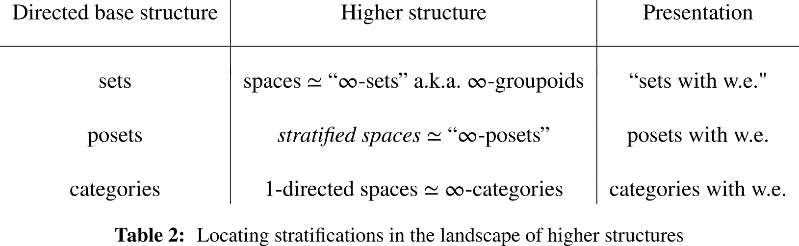
Simple enough! But, if you happen to have an inclination towards higher structures, then I can easily relay a better way of thinking about stratifications in a single sentence: namely, spaces are to sets, what stratified spaces are to posets. The situation is illustrated in Table 2 (non-standard terminology is kept in quotes as before). In particular, just as spaces have fundamental sets , stratified spaces have fundamental posets . Just as spaces have fundamental -groupoids , and both and model the same homotopy type, stratified spaces have fundamental -posets , and both model the same higher structure. (Here ‘’ indicates that in the literature one more commonly finds the terms ‘Entrance’ or ‘Exit path categories’; but really, there’s a general story to be told here for passing from a structure S to an -S structure, and from a topological thing to its fundamental category, so ‘fundamental -poset’ is not a bad name at all and it illustrates the point.) Importantly, to make this higher-categorical story work nicely, it turns out to be central that our topological definition of stratified spaces has one further property: conicality!
While both conicality and the aforementioned higher-categorical constructions are discussed in more detail in the extended version of this post, here, we shall not need them in full generality. Indeed, we are only interested in the framed euclidean case, and that case goes as follows.
First, note that the adjectives ‘framed’ and ‘stratified’ can be easily combined: for instance, a framed stratified map is a stratified map whose underlying map is framed. Moreover, when working with stratified products we will identitify in the standard way; and, when working with stratified cones of stratified spaces , we will standard embed and identify by mapping to .
With these conventions at hand, we may now introduce conicality in our framed setting as follows: a stratification is framed conical if each point has a framed stratified neighborhood for which we may choose and a stratification such that there exists a framed stratified homeomorphism
and (under this homeomorphism) is mapped into . (Note that the stratification is also called a link around .) Importantly, framed conicality is really just a ‘framed’ version of traditional conicality!
Ingredient 3: Framed compact triangulability
The last ingredient for the notion of manifold diagrams is that of framed compact triangulability. To begin, let me remark that imposing a compact triangulability condition is a reasonable thing to do: indeed, in our earlier discussion of Pontryagin’s theorem we met cobordisms of manifolds embedded in that have compact support — ‘framed compact triangulability’ may be thought of as a generalization of this situation (adapted to the setting of framed stratifications). The condition can be succinctly formulated by starting in the PL category: a compactly-defined triangulation of is a finite stratification of by open disks whose closures are the images of linear embeddings (where ). This translates to the framed stratified case as follows: a stratification is framed compactly triangulable if it admits a framed stratified subdivision of by a compactly-defined triangulation . (Note, a ‘subdivision’ is a stratified map whose underlying map is a homeomorphism.)
Putting it all together
We have now introduced all the necessary ingredients (and importantly, there are not that many), and we can mix them together in the following central definition.
Definition ([4]). A manifold -diagram is a framed conical stratification that is framed compactly triangulable.
Let’s unwind this definition and look at some examples. First, in order to be able to depict , observe that there is a framed homeomorphism ; here, ‘framed’ means that composing with the inclusion yields a framed map as defined earlier (in fact, the choice for a framed identification is again unique up to contractible choice). With that in mind, we will depict all our examples of manifold diagrams as living on the open cube .
Example 1: String diagrams. An ordinary string diagram is a manifold 2-diagram. We illustrate one in Figure 1 below, and visually verify the framed conicality condition at three points.
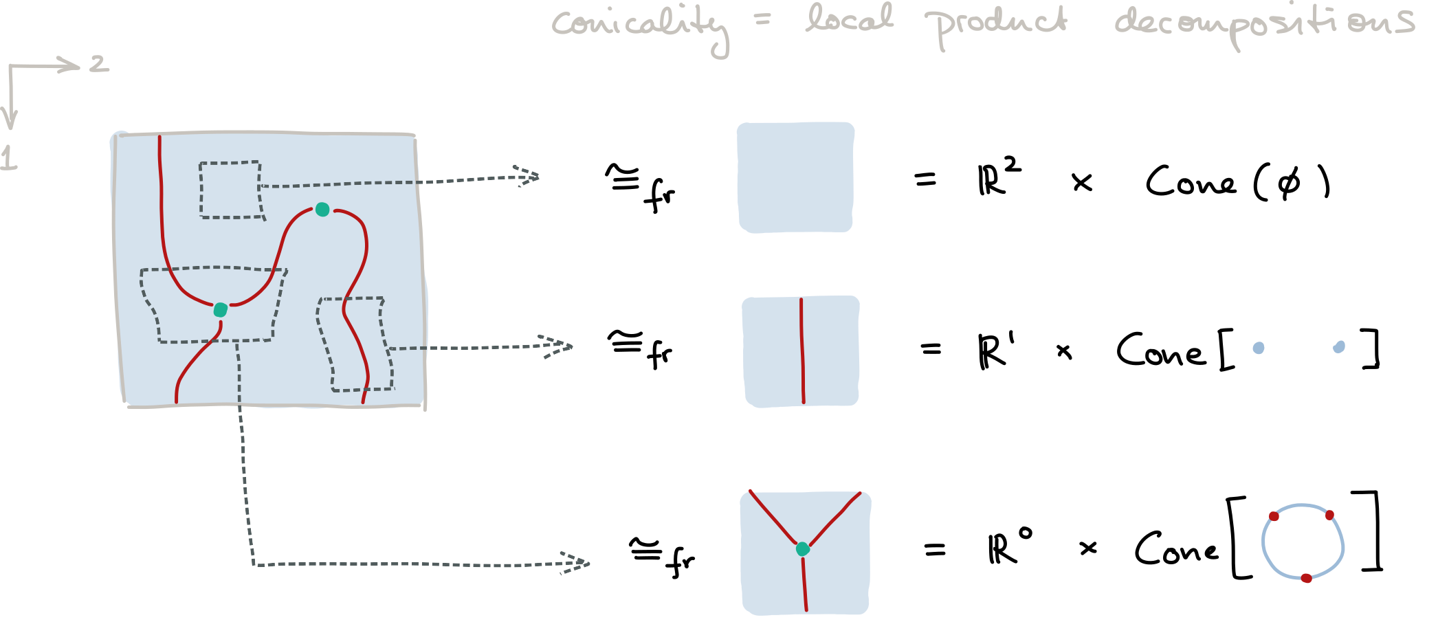
Figure 1: A manifold 2-diagram or ‘string diagram’.
Example 2: The ‘Cockett pocket’ composite (Verity). Consider the stratification shown in Figure 2 below: this is a manifold 3-diagram. We indicate a tubular neighborhood and its framed conical structure as before.
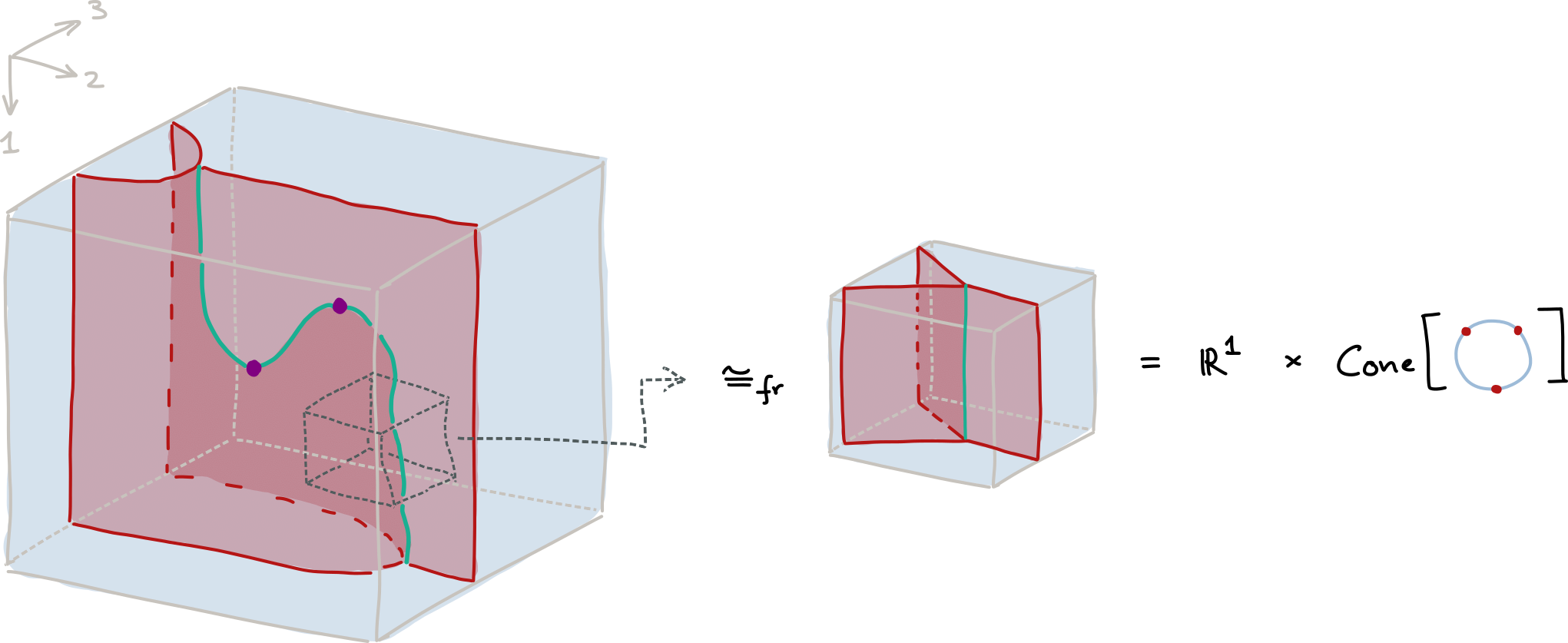
Figure 2: A manifold 3-diagram or ‘surface diagram’.
Example 3: -series singularities. It is often useful to think of a manifold -diagram as a ‘movie’ of manifold -diagrams. As an example, check out this Lab picture: the first surface illustrates a manifold 3-diagram as a movie of manifold 2-diagrams (note that the diagram is ‘stratified by the named strata’; for instance, the surface labelled by is its own stratum, and so is the line stratum labeled by etc.). One dimension up, we can similarly depict manifold 4-diagrams as movies of manifold 3-diagrams: for instance, Figure 3 below shows a movie that starts with the 3-diagram we’ve just seen, and then gradually shrinks its ‘interior’ into a point.
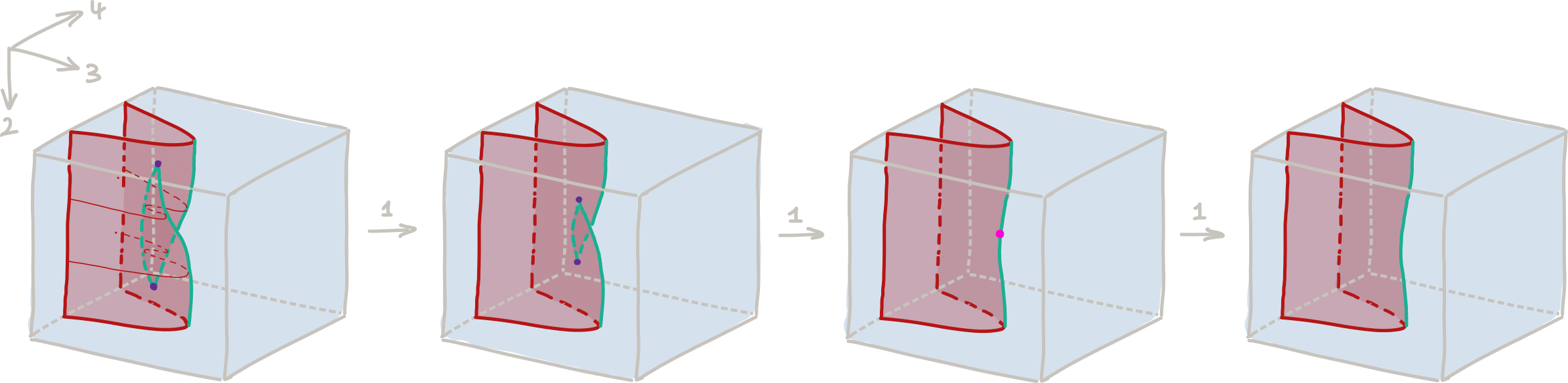
Figure 3: The ‘swallowtail’, or A3 singularity, as a manifold 4-diagram.
In fact, this is manifold 4-diagram has a name: it’s often called the ‘swallowtail’ and it corresponds to the classical differential singularity; as such, it is part of an infinite series of so-called singularities! Bonus trivia: the linked picture happens to be the title image of MSRI program 323 “Higher categories and categorification”.
Example 4: -series singularities. There is a bigger story to be told about ‘singularities’: roughly speaking, singularities are those manifold -diagrams in which we can merge strata into a single embedded -manifold that is then framed stratified homeomorphic to the cone of an embedding . The swallowtail mentioned above provides one example. Interestingly, one also finds examples that do not have classical differential counterparts (in that they don’t directly arise as (parametrized) graphs of (parametrized) smooth functions, see [4, Sec. 3.4] for the heuristic idea at play). The first such non-classical singularity is the ‘’ singularity (for the experts: this corresponds to the ‘horizontal cusp’ movie move in Carter-Saito’s work), and it is illustrated in Figure 4 below.
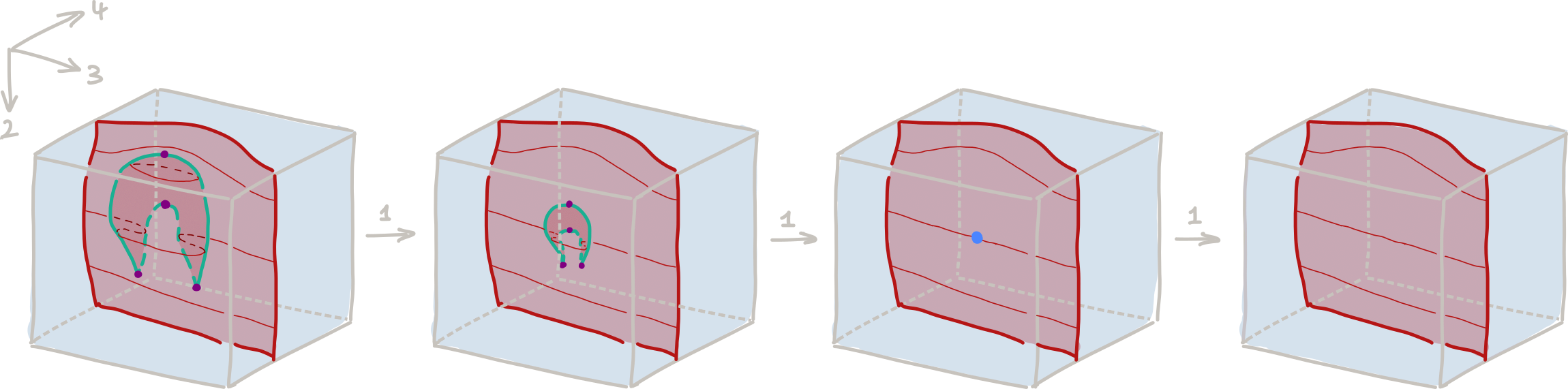
Figure 4: The manifold 4-diagram of the D2 singularity.
One dimension up, the singularity itself becomes part of the link of other singularities. One of these, termed the singularity (which, again, is a non-classical singularity), is particularly interesting and its link is given by the movie in Figure 5 (the full manifold 5-diagram is a movie of movies, which shrinks the interior of the given movie into a single point… similar to Figure 3 and 4, but one dimension higher!)
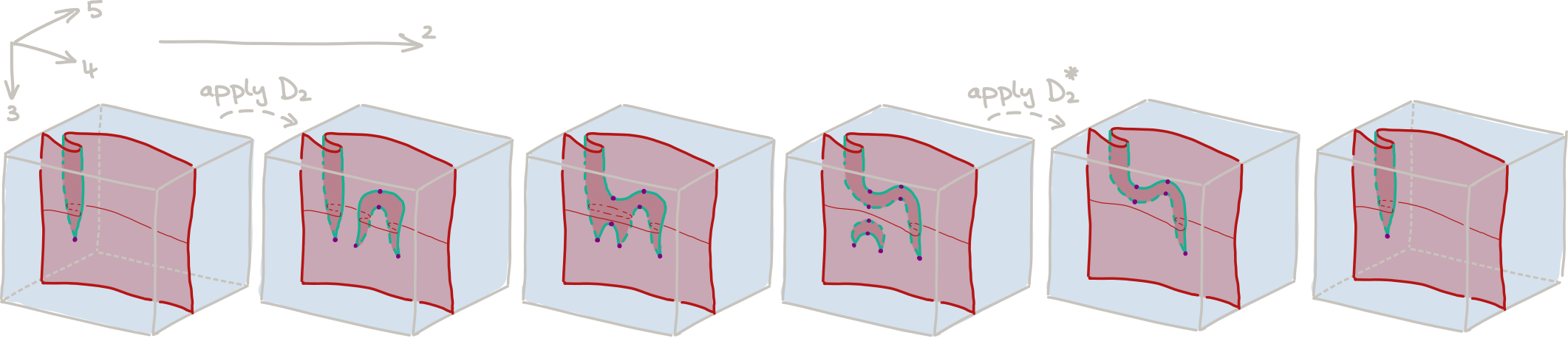
Figure 5: The D3 singularity link as a manifold 4-diagram (containing two D2 singularities).
Even one dimension up from (now working in !), we find singularities whose link contains singularities, and (surprise!) one of these now corresponds to the classical differential singularity (which, again, is only the beginning of an infinite sequence of so-called singularities). In Figure 6, we depict the -projection (namely, projecting along the standard projection which forgets the last three coordinates) of certain strata in , and a comparison to other singularities in that dimension. However, for any substantive discussion of these pictures and symbols we must refer to [4, Sec. 3.4] and this post. (A vatic aside: the reason that we can so confidently work in all dimensions, ultimately, roots in the combinatorial dimension-inductive principles secretly controlling manifold diagrams in the background … see ‘property (1)’ below!)
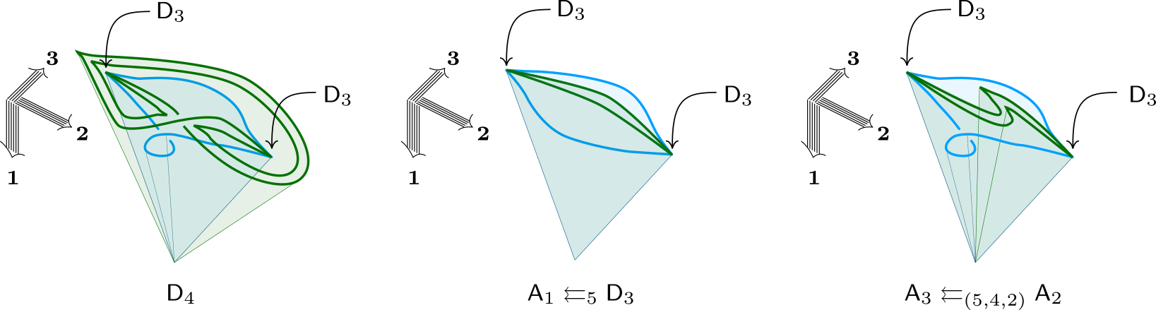
Figure 6: 3-projections of the manifold 6-diagram D4 singularity and other singularities in dim 6.
Example 5: Braids, Reidemeister III and beyond. Besides singularities, manifold diagrams also describe interesting ‘interactions at a distance’ of manifold strata. The braid provides a first example of this: as illustrated in Figure 7, it is a manifold 3-diagram which tracks two points in the plane rotating around one another by . (You should check that not only is the braid a manifold diagram, but it is not framed stratified homeomorphic to any product diagram , where the second factor is a stratification of the plane by two embedded points and their complement.)
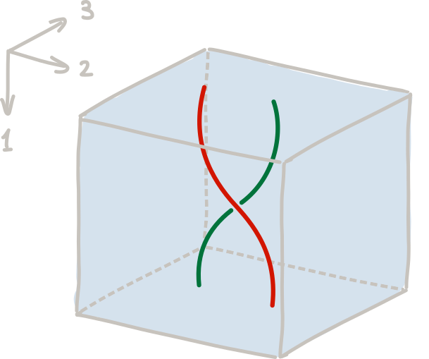
Figure 7: The braid isotopy.
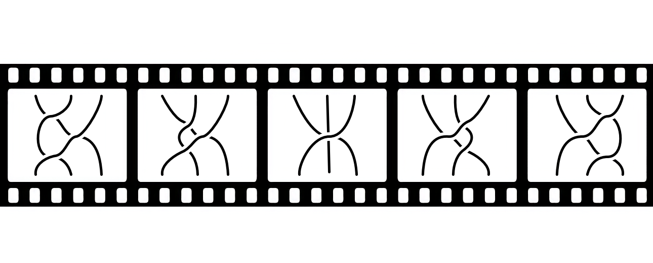
One dimension up, we find the Reidemeister III isotopy, which is the (track of an) isotopy that shifts a constellation of three braids into a different constellation of three braids, while passing through a ‘triple braid’. This is illustrated in this Lab picture and it, too, is a manifold 4-diagram as can be easily verified! And, in yet higher dimensions, you will start seeing isotopies such as the Zamolodchikov tetrahedron identity cropping up as manifold diagrams. We will briefly return to the topic of isotopies later!
The first few properties
Let us mention a few important consequences of our definition of manifold diagrams, some of which link back to our earlier question of why one may want to care about manifold diagrams, and others which highlight some of the pleasant properties of manifold diagrams (the verifications of all these claims can be found in [4]).
(1) Canonical combinatorializations. While the compact triangulability condition requires the existence of some combinatorial representation (namely a triangulation), it turns out that there is in fact a canonical combinatorial representation for manifold diagrams (up to framed stratified homeomorphism).
For the experts, it may be helpful to give a somewhat condensed explanation here: the claim follows from the observation that manifold -diagrams have coarsest framed subdivisions by certain projection-stable stratified 0-types called -meshes (where ‘stratified 0-type’ means that the -poset is equivalent to a poset, and ‘projection-stable’ means that projects onto a -mesh). Meshes, in turn, are fully described by their ‘framed’ fundamental posets , also called trusses. Finally, trusses (endowed with appropriate combinatorial stratification data) combinatorially classify manifold diagrams. The process is illustrated in Figure 8.
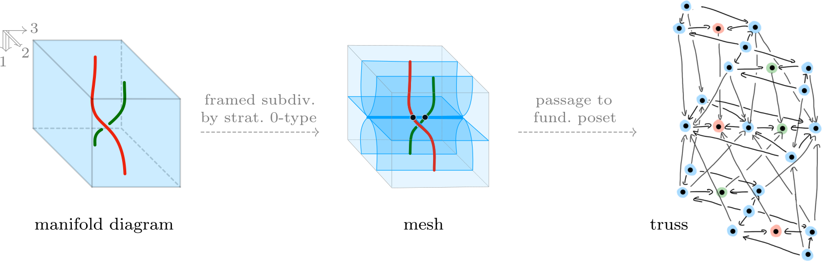
Figure 8: The braid, its canonical mesh, and its combinatorializing truss.
(2) Manifold regularity. Strata in manifold diagrams are, indeed, manifolds (this is an immediate consequence of the framed conicality condition). However, more turns out to be true: strata have canonical smooth structures as well! This follows since strata inherit a classical framing (from the framing of the ambient Euclidean space), since all strata in manifold diagrams are PL manifolds (this follows at root from the theory behind point (1)), and since, by smoothing theory, framed PL manifolds have unique framed smooth structure.
(3) Link well-definedness. Links of strata found in manifold diagrams (i.e. the stratifications with symbol ‘’ in the earlier definition) are in fact well-defined: that is, there is, up to framed stratified homeomorphism, a unique choice of link at any given point of the diagram. This stands in contrast to classical topological conical stratifications, where non-homeomorphic choices of links exist.
(4) Geometric duality. Manifold diagrams have canonical geometric duals (in the sense of Poincaré duality). This duality relates manifold diagrams to so-called (framed) cell diagrams, which may then be considered as classical pasting diagrams (but with cells whose shapes generalize most of the familiar classes of shapes, such as ‘globular’, ‘simplicial’, or ‘opetopic’ shapes).
Let me dwell, and highlight once more, point (1) of the above list for a moment. It turns out that, as a consequence of (1), essentially all parts of the theory manifolds diagrams (i.e. their mappings, their neighborhoods, their links, their products, their cones, etc.) have canonical combinatorial counterparts in the theory of trusses — this quickly leads us on a path into a rich combinatorial world, which is explored in some detail in [3, Ch. 2] (and to which I also devoted (way too) many pages in my PhD thesis). Moreover, many parts of this combinatorial world are, in contrast to classical PL combinatorics, computationally tractable, which then extends to computability statements about manifold diagrams as well: for instance, the ‘framed stratified homeomorphism problem’ for manifold -diagrams is decidable, while the analogous ‘stratified (PL) homeomorphism problem’ for compact PL stratifications in is undecidable. (In fact, this observation is implicitly exploited by the diagrammatic proof assistant homotopy.io!) In summary, as a consequence of (1), manifold diagrams become very tractable objects to work with.
Geometric computads and beyond
With the central definition of manifold diagrams spelled out, let us begin to wrap things up and end this post by pointing out a few further directions of research (if you feel that this ending is premature, once more, I happily refer you to the extended version of this post!). Let’s start with a closer look at point (4) from the above list as it, too, entails an interesting story. The geometric duality of manifold and cell diagrams is parallel to (in fact, it is based on) a geometric duality in the theory of meshes (which, at the level of framed fundamental posets, becomes a categorical duality in the theory of trusses). The ‘dual meshes’ produced in this way turn out to be cell complexes: their cells are characterized by being both regular and carrying compatible framings — accordingly, they have been termed framed regular cells in [3]. Dualizing the observation of manifold diagrams admitting canonical subdivisions into meshes, one finds that cell diagrams equally have canonical subdivisions into framed regular cell complexes (these are the ‘dual meshes’). However, this subdivision is a non-identity stratified map and it carries important information: it records which cells belong to the same stratum, or, in categorical terms, it records which cells are secretly degeneracies of lower dimensional cells. The ‘stratified encoding’ of degeneracies in this way may be a bit unfamiliar, but, together with the large shape class of framed regular cells, it has powerful consequences.
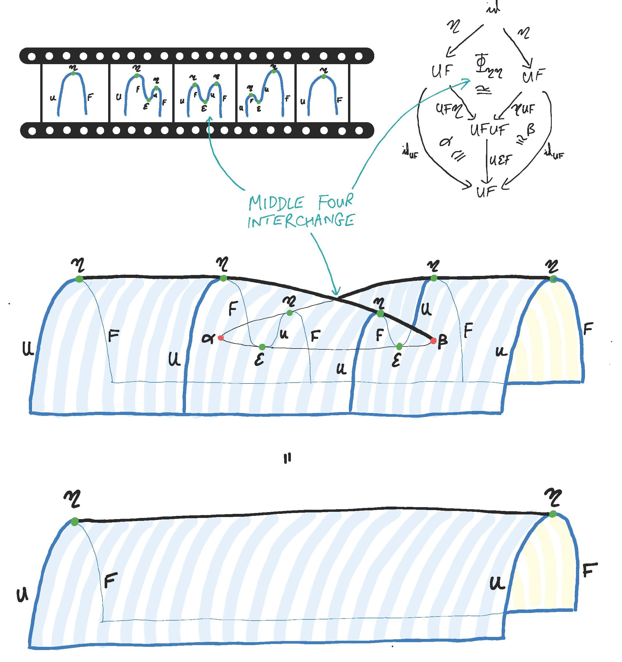
Manifold -diagrams that do not contain point strata are also called diagram isotopies. They may be thought of as the tracks of ordinary stratified isotopies of manifold -diagrams (the braid, which we met in Figure 7, is an example). It has been a long held intuition that such isotopies encode certain higher-categorical coherences. The translation underlying this intuition (from isotopies to higher-categorical laws) can be made fully precise via point (4): indeed, dualization translates isotopies to certain cell diagrams, which, after accounting for degeneracies, can then be cast as an equation between pasting diagrams. (It may be equally remarkable to note that the combinatorializability of manifold diagrams leads to a fully combinatorial theory of isotopies of manifold diagrams in the first place.) My favorite example of this process is the definition of categorical laws governing the sequence of categories, functors, natural transformations, modifications, … .
With a notion of directed cells at hand, we may also consider ‘global’ directed higher structures simply by appropriately gluing such cells. The simplest, but also most instructive, such construction happens when we build our higher structures freely: this yields the case of geometric computads. The definition of geometric computads is exceedingly simple, as it need not follow the traditional inductive two-step procedure of building computads: indeed, usually one constructs computads inductively by, in the th step, adding generating -morphisms with boundary in existing -morphisms, and then passing to the closure under composition and coherence conditions (which, passing back and forth between “new composites” and “new coherences” is often a pretty infinite process). In geometric computads, this is process becomes unnecessary: boundaries of -morphisms are manifold -diagrams (or, if you work dually, cell -diagrams) which already can express all the composites and isotopies you could possibly need. This makes geometric computads really easy to work with.
The story of geometric higher structures can be spun further in various ways, and active development of its foundations is still underway. One direction that I wanted to highlight (in fact, asking David Corfield about this direction was the original motivation for writing the present blog post) is geometric higher type theory: basically, the idea is to exploit the easiness of geometric computads and their isotopy coherence laws in order to study the “internal language of the geometric computad of all geometric computads”. A hypothetical higher type theory of this kind could have interesting consequences, for instance, by demonstrating that types can be internally constructed from a set of basic higher compositional principles (i.e. they need not be assumed as primitive rules). But, in only the last two sentences, we have gotten ourselves into rather speculative terrain!
Finally, one of my favorite and dearest parts of geometric higher categorical thinking (which, at the same time, is also one of the most mysterious parts for me) is the role that invertibility and dualizability plays in it. Here, of course, the cobordism hypothesis finally comes into play: invertible morphisms are modelled not by manifold diagrams, but by so-called tangle diagrams — (omitting all details,) tangle diagrams are simply a variation of manifold diagrams in which we allow strata to ‘change directions’ with respect to the ambient framing [4]. However, really, this set-up leads to a rather refined perspective on tangles as it provides a combinatorial framework for studying neighborhoods of ‘higher critical points’ (i.e. the points where tangles ‘change direction’). There is a tantalizing but mysterious connection of these critical points with classical differential ADE singularities [2]: on one hand, classical singularities seem to resurface as ‘perturbation-stable’ singularities in tangle diagrams, on the other hand, the differential machinery breaks down (producing ‘moduli of singularities’) in high parameter ranges and this simply cannot happen in the combinatorial approach; put differently, the combinatorial approach must be better behaved than the differential approach in some way. Certainly, the ‘higher compositional’ perspective given through the lens of diagrams is something that also has no differential counterpart at all (and it leads to new interesting observations, for instance, how to break up the classical three-fold symmetry of into a bunch of binarily-paired-up singularities, as we visualized in Figure 6). But despite many ‘visible patterns’, most of this line of research remains completely unexplored (attempts of laying at least some foundations were made in [4])… but maybe that’s what I find so exciting about it. :-)
These are just a few of many directions you could pursue in studying geometric higher categories. And I hope with time, the picture of how geometric higher categories might contribute to the larger endeavours of current research in mathematics and physics will become clearer.
Acknowledgments
I would really like to take this opportunity to thank the hosts of the -Category Café, which has been, and continues to be, a source of inspiration in manifold aspects of research and life. In particular, many of the ideas in geometric higher category theory have been thought up by you. And many other ramblings have been very fun to read. (And while I’m at it, let me also give a shout out to the currently or formerly Oxford-based thinkers of geometric higher categories: Christopher Douglas, Lukas Heidemann, André Henriques, David Reutter, Jamie Vicary, and many others, all of whose work has contributed to this area slowly emerging over the past few years).
An incomplete list of references
[1] Buoncristiano, Rourke and Sanderson. A geometric approach to homology theory. 1976. (CUP, ResearchGate)
[2] Arnold. Normal forms for functions near degenerate critical points, the Weyl groups of , , and Lagrangian singularities. 1972. (Springer)
[3] Dorn and Douglas. Framed combinatorial topology. 2021. (arXiv, latest)
[4] Dorn and Douglas. Manifold diagrams and tame tangles. 2022. (arXiv, latest)
Re: An Invitation to Geometric Higher Categories
Thanks, Christoph! Plenty to talk about there.
Back in the day, there was lots of talk of the difference between algebraic and non-algebraic/topological approaches to -categories. E.g., here’s a picture from Tom Leinster’s A Perspective on Higher Category Theory on the homotopy hypothesis:
So now we’re hearing of a third pole, the geometric.
If I recall we only heard about this geometric pole in the context of -categories with duals, back in this thread that you alluded to. Was this an artifact of considering paths entering and exiting through the strata?
I recall there was a uni-directed approach by Jon Woolf. I mention it here, and Jon replies. Yes, so just an exiting through strata.