Skip to the Main Content

Note:These pages make extensive use of the latest XHTML and CSS Standards. They ought to look great in any standards-compliant modern browser. Unfortunately, they will probably look horrible in older browsers, like Netscape 4.x and IE 4.x. Moreover, many posts use MathML, which is, currently only supported in Mozilla. My best suggestion (and you will thank me when surfing an ever-increasing number of sites on the web which have been crafted to use the new standards) is to upgrade to the latest version of your browser. If that's not possible, consider moving to the Standards-compliant and open-source Mozilla browser.

May 17, 2022

The Magnitude of Information

Posted by Tom Leinster

Guest post by Heiko Gimperlein, Magnus Goffeng and Nikoletta Louca

The magnitude of a metric space (X,d)(X,d) does not require further introduction on this blog. Two of the hosts, Tom Leinster and Simon Willerton, conjectured that the magnitude function X(R):=Mag(X,Rd)\mathcal{M}_X(R) := \mathrm{Mag}(X,R \cdot \mathrm{d}) of a convex body X nX \subset \mathbb{R}^n with Euclidean distance d\mathrm{d} captures classical geometric information about XX:

X(R)= 1n!ω nvol n(X)R n+12(n1)!ω n1vol n1(X)R n1++1 = 1n!ω n j=0 nc j(X)R nj\begin{aligned} \mathcal{M}_X(R) =& \frac{1}{n! \omega_n} \mathrm{vol}_n(X)\ R^n + \frac{1}{2(n-1)! \omega_{n-1}} \mathrm{vol}_{n-1}(\partial X)\ R^{n-1} + \cdots + 1 \\ =& \frac{1}{n! \omega_n} \sum_{j=0}^n c_j(X)\ R^{n-j} \end{aligned}

where c j(X)=γ j,nV j(X)c_j(X) = \gamma_{j,n} V_j(X) is proportional to the jj-th intrinsic volume V jV_j of XX and ω n\omega_n is the volume of the unit ball in n\mathbb{R}^n.

Even more basic geometric questions have remained unknown, including:

  • What geometric content is encoded in X\mathcal{M}_X?
  • What can be said about the magnitude function of the unit disk B 2 2B_2 \subset \mathbb{R}^2?

We discuss in this post how these questions led us to possible relations to information geometry. We would love to hear from you:

  • Is magnitude an interesting invariant for information geometry?
  • Is there a category theoretic motivation, like Lawvere’s view of a metric space as an enriched category?
  • Does the magnitude relate to notions studied in information geometry?
  • Do you have interesting questions about this invariant?

(a) Cylinder, (b) spherical shell, (c) spherical cap, (d) ball in hyperbolic plane (hyperboloid model), (e) toroidal armband.

Recent years have seen much progress to understand the geometric content of the magnitude function for domains in odd-dimensional Euclidean space. In this setting Meckes and Barceló–Carbery showed how to compute magnitude using differential equations. Nevertheless, as Carbery often emphasized, hardly anything was known even for such simple geometries as the unit disk B 2B_2 in 2\mathbb{R}^2.

Our new works Semiclassical analysis of a nonlocal boundary value problem related to magnitude and The magnitude and spectral geometry show, in particular, that as RR\to \infty,

B 2(R)=12R 2+32R+98+O(R 1),\mathcal{M}_{B_2}(R) = \frac{1}{2}R^2 + \frac{3}{2}R + \frac{9}{8}+O(R^{-1}),

and that B 2(R)\mathcal{M}_{B_2}(R) is not a polynomial.
The approach does not use differential equations, but methods for integral equations. Recall that the magnitude of a positive definite compact metric space (X,d)(X,\mathrm{d}) is defined as

(X,D)(R):= Xu R(x)dx,\mathcal{M}_{(X,D)}(R):=\int_X u_R(x) \ \mathrm{d}x,

where u Ru_R is the unique distribution supported in XX that solves the integral equation

Xe Rd(x,y)u R(y)dy=1.\int_X \mathrm{e}^{-R\mathrm{d}(x,y)}u_R(y) \ \mathrm{d}y=1.

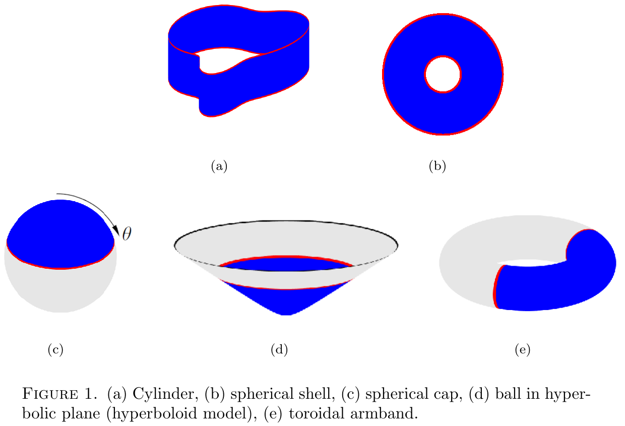
We analyze this integral equation in geometric settings, for domains XX in n\mathbb{R}^n, in spheres, tori or, generally, a manifold with boundary with a distance function of any dimension, as illustrated in the figures above. Our results shed light on the geometric content of their magnitude. In fact, our results apply beyond classical geometry and metric spaces — not even a distance function is needed!

Our techniques suggest a life of magnitude beyond metric spaces in information geometry. There one considers a statistical manifold, i.e. a smooth manifold XX with a divergence DD, not with a distance function: See John Baez’s posts on information geometry. A first example of a divergence is the square of the subspace distance |xy| 2|x-y|^2 on a submanifold in Euclidean space. A second example is the square of the geodesic distance function on a Riemannian manifold (X,g)(X,g), provided that it is smooth. (Note that on a circle the distance function and its square are non-smooth when xx and yy are conjugate points.) In general, a divergence D=D(x,y)D=D(x,y) is a smooth, non-negative function such that DD is a Riemannian metric near x=yx=y modulo lower order terms, in the sense that

D(x,x+v)=g D,x(v,v)+O(|v| 3) D(x,x+v)=g_{D,x}(v,v)+O(|v|^3)

for a Riemannian metric g Dg_D on XX.

Divergences related to relative entropy have long been used in statistics to study families of probability measures. The relative entropy of two probability measures μ\mu and ν\nu on a space Ω\Omega is defined as

D(μ,ν):= Ωlog(dνdμ)dν[0,].D(\mu,\nu):=\int_\Omega \log\left(\frac{\mathrm{d}\nu}{\mathrm{d}\mu}\right)\mathrm{d}\nu\in [0,\infty].

The notion of relative entropy and its cousins are discussed in the blog posts of Baez mentioned above and also in Leinster’s book Entropy and Diversity: The Axiomatic Approach. While the space of probability measures is too big, one can restrict to interesting submanifolds (with boundary).

Here is the definition of the magnitude function of a statistical manifold with boundary (X,D)(X,D), when R0R \gg 0 is sufficiently large:

(X,D)(R):= Xu R(x)dx,\mathcal{M}_{(X,D)}(R):=\int_X u_R(x) \ \mathrm{d}x,

where u Ru_R is the unique distribution supported in XX that solves the integral equation

Xe RD(x,y)u R(y)dy=1.\int_X \mathrm{e}^{-R\sqrt{D(x,y)}}u_R(y) \ \mathrm{d}y=1.

When DD is the square of a distance function on XX, we recover the magnitude of the metric space (X,D)(X,\sqrt{D}).

We emphasize two key points to take home:

  1. The integral equation approach is equivalent to defining the magnitude of statistical manifolds using Meckes’s classical approach in Magnitude, diversity, capacities, and dimensions of metric spaces, relying on reproducing kernel Hilbert spaces.

  2. Since DD is smooth, (X,D)\mathcal{M}_{(X,D)} shares the properties stated in The magnitude and spectral geometry for the magnitude function summarized next.

Theorem

a. The magnitude is well-defined for R0R\gg 0 sufficiently large; there the integral equation admits a unique distributional solution.

b. (X,D)\mathcal{M}_{(X,D)} extends meromorphically to the complex plane.

c. The asymptotic behavior of (X,D)(R)=1n!ω n j=0 c j(X)R nj+O(R )\mathcal{M}_{(X,D)}(R) = \frac{1}{n! \omega_n} \sum_{j=0}^\infty c_j(X) R^{n-j}+O(R^{-\infty}) is determined by the Taylor coefficients of vD(x,x+v)v\mapsto D(x,x+v) and n=dimXn=\mathrm{dim} X.

Further details and explicit computations of the first few terms c jc_j(X) can be found in The magnitude and spectral geometry: For a Riemannian manifold c 0c_0 is proportional to the volume of XX, while c 1c_1 is proportional to the surface area of X\partial X. c 2c_2 involves the integral of the scalar curvature of XX and the integral of the mean curvature of X\partial X. All these computations are relative to DD and the Riemannian metric that DD defines. For Euclidean domains X nX \subset \mathbb{R}^n, c 3c_3 is proportional to the Willmore energy of X\partial X (proven with older technology in another paper: The Willmore energy and the magnitude of Euclidean domains). We note that

in all known computations of asymptotics for Euclidean domains X nX \subset \mathbb{R}^n, c j(X)c_j(X) is proportional to XH j1dS\int_{\partial X}H^{j-1}\mathrm{d}S for j>0j\gt 0.

Here HH denotes the mean curvature of X\partial X. You can compute lower-order terms by an iterative scheme, for as long as you have the time. In fact, we have written a python code which computes c jc_j for any jj, which is available at arXiv:2201.11363.

We would love to hear from you should you have any thoughts on the following questions:

  • Is magnitude an interesting invariant for information geometry?

  • Is there a category theoretic motivation, like Lawvere’s view of a metric space as an enriched category?

  • Does the magnitude relate to notions studied in information geometry?

  • Do you have interesting questions about this invariant?

Posted at May 17, 2022 11:44 AM UTC

TrackBack URL for this Entry:   https://golem.ph.utexas.edu/cgi-bin/MT-3.0/dxy-tb.fcgi/3397

10 Comments & 0 Trackbacks

Re: The Magnitude of Information

There’s loads of good stuff here, but let me highlight one particular point: finally, we know something about the magnitude of a Euclidean disc!

Some context:

  • We’ve known from the start that the magnitude of a 1-dimensional ball — that is, a line segment — is a polynomial of degree 1 in its radius (or length).

  • Juan Antonio Barceló and Tony Carbery showed that the magnitude of a 3-dimensional ball is a polynomial of degree 3 in its radius.

  • They also showed that in odd dimensions d5d \geq 5, the magnitude of a dd-dimensional ball is a rational function in the radius, but not a polynomial.

  • And we’ve known for a long time that for every dd, the magnitude of the dd-dimensional ball of radius RR grows like R dR^d as RR \to \infty. This explains the degrees of the polynomials just mentioned.

What we didn’t know much about until Heiko, Magnus and Nikoletta’s work is the magnitude of even-dimensional balls. As they say in the post above, the 2-dimensional ball of radius RR has magnitude

12R 2+32R+98+O(R 1) \frac{1}{2}R^2 + \frac{3}{2} R + \frac{9}{8} + O(R^{-1})

as RR \to \infty, and it’s not a polynomial in RR!

So we have a funny situation:

  • the magnitude of a 1-dimensional ball is a polynomial in its radius;

  • the magnitude of a 3-dimensional ball is a polynomial in its radius;

  • but the magnitude of a 2-dimensional ball is not.

I have a very rough idea of why that’s the case, but really not what you could call a conceptual explanation. Finding a conceptual explanation seems like a real challenge.

Posted by: Tom Leinster on May 18, 2022 12:11 AM | Permalink | Reply to this

Re: The Magnitude of Information

You’ve shown that the magnitude function of a 2-disc is not a polynomial. Do you know whether it’s a rational function?

Posted by: Tom Leinster on May 18, 2022 12:16 AM | Permalink | Reply to this

Re: The Magnitude of Information

Unfortunately, our methods do not allow us to say whether or not the magnitude function of the unit disk is rational.

Except for odd-dimensional balls little seems known about algebraic properties of the magnitude function. The simple formulas for the first expansion coefficients c j(X)c_j(X) of a general domain XX in n\mathbb{R}^n (see the bold-faced “note” after the theorem) might hint at interesting, but hidden structure.

Posted by: Heiko Gimperlein on May 18, 2022 6:12 AM | Permalink | Reply to this

Re: The Magnitude of Information

Thanks.

I wonder whether Simon has thoughts on what rational function it might be if it is a rational function, given the intensive study he’s done of the coefficients of these functions for odd-dimensional balls.

Posted by: Tom Leinster on May 18, 2022 9:34 AM | Permalink | Reply to this

Re: The Magnitude of Information

Looking at the information geometry aspect of this post, I see that there’s a very simple question to which I don’t know the answer. I’m guessing no one does, but please correct me if I’m wrong.

Take the unit interval [0,1][0, 1]. We know its magnitude with respect to the usual distance. But what is its magnitude if we replace the usual distance by the square root of relative entropy, regarding [0,1][0, 1] as the set of probability distributions on a two-element set? In other words, for p,q[0,1]p, q \in [0, 1], we’re replacing |pq||p - q| by

ρ(p,q):={plog(pq)+(1p)log(1p1q)} 1/2. \rho(p, q) := \left\{ p \log \biggl( \frac{p}{q} \biggr) + (1 - p) \log \biggl( \frac{1 - p}{1 - q} \biggr) \right\}^{1/2}.

Or, as usual, we can ask the same question with a scale factor introduced, i.e. replacing ρ(p,q)\rho(p, q) by Rρ(p,q)R \rho(p, q) for a variable factor R>0R \gt 0.

I think this is the simplest case of the question that Heiko, Magnus and Nikoletta are asking towards the end of the post.

The theorem there gives us some information, but only some. E.g. it tells us that the large-RR asymptotics of the magnitude function are the same as those of an ordinary interval, right? But perhaps we can say something about non-large RR. Perhaps there’s even a closed form formula.

Posted by: Tom Leinster on May 22, 2022 10:58 AM | Permalink | Reply to this

Re: The Magnitude of Information

Thanks for this interesting question Tom!

At the current state of affairs, there might be more hope for explicit computations in this example than any statements from our methods. The example you give is not smooth in the end points q=0 and q=1, so our methods can not say anything about the boundary terms in that case. The methods can describe the interior behavior (up to arbitrary order of R), and provide complete asymptotics on any proper subdomain [ϵ,1δ][\epsilon,1-\delta]. Perhaps I am overly negative, but the endpoints would require heavier hammers than we are wielding.

From a bigger perspective, it might be that your example showcases a potential issue with applications of magnitude to information geometry: that the extreme points do not behave that nice in a divergence sense. Or am I extrapolating too much from your example?

Posted by: Magnus Goffeng on May 22, 2022 7:25 PM | Permalink | Reply to this

Re: The Magnitude of Information

No, I agree, the boundary is potentially a real issue.

To explain why, let me back up a bit. I suspect I’m about to say some stuff you already know, Magnus, but I’ll say it anyway.

For any Riemannian manifold M=(M,g)M = (M, g), and any point pp of MM, we have a function

d(,p) 2:M, d(-, p)^2: M \to \mathbb{R},

where dd is the geodesic distance derived from the Riemannian metric gg. This function is smooth in a neighbourhood of pp, so we can take its Hessian

Hess p(d(,p) 2), Hess_p(d(-, p)^2),

which is a bilinear form on the tangent space T pMT_p M. But the original metric gg itself also gives a bilinear form on T pMT_p M — namely, g pg_p. These two forms are essentially equal:

g p=12Hess p(d(,p) 2). g_p = \frac{1}{2} Hess_p(d(-, p)^2).

The point of this equation is that it expresses the infinitesimal metric gg in terms of the global metric dd.

(What I’ve just said seems to be obvious to Riemannian geometers, but I’ve never succeeded in finding a reference where it’s expressed this directly. It’s done on p.78 of my book.)

Now here’s the main thought. If we have some roughly distance-like thing δ\delta that nevertheless doesn’t satisfy the metric space axioms, we can still use the formula

g p=12Hess p(δ(,p) 2) g_p = \frac{1}{2} Hess_p(\delta(-, p)^2)

to define a Riemannian metric gg. So from a “fake” distance function δ\delta, we derive a genuine Riemannian metric gg. And from gg, we can construct its geodesic distance function dd, which does satisfy the metric space axioms.

(Aside: I’d love to see a purely elementary version of the construction δd\delta \mapsto d that doesn’t refer to the manifold structure or any kind of smoothness.)

The point of all this is that you can take δ\delta to be the square root of relative entropy on the manifold Δ n \Delta_n^\circ of probability distributions on {1,,n}\{1, \ldots, n\} of full support. And when we do this, the process just described spits out a genuine metric on Δ n \Delta_n^\circ, called the Fisher metric. Up to a scale factor, it makes Δ n \Delta_n^\circ isometric to the positive orthant

S + n1:=S n1(0,) n S^{n - 1}_+ := S^{n - 1} \cap (0, \infty)^n

of the unit sphere with its geodesic metric. The isometry makes a probability distribution (p 1,,p n)(p_1, \ldots, p_n) correspond to a point (p 1,,p n)(\sqrt{p_1}, \ldots, \sqrt{p_n}) of the sphere.

That’s all standard stuff in information geometry. But notice that the words “full support” snuck in. They mean that none of the probabilities are 00, so Δ n \Delta_n^\circ is an open simplex. If we allowed zero probabilities, it would be a manifold with boundaries, and not an honest manifold.

My impression is that this point requires care. For instance, the book Information Geometry of Ay, Jost, Lê and Schwachhöfer has a section called “Extending the Fisher metric to the boundary” (p. 33), which begins like this:

As is obvious from (2.13) and also from the first fundamental form (2.19), the Fisher metric is not defined at the boundary of the simplex. It is, however, possible to extend the Fisher metric to the boundary…

So even these experts in information geometry define the Fisher metric in a two-step process, first on the interior and then extending to the boundary.

Posted by: Tom Leinster on May 23, 2022 11:25 AM | Permalink | Reply to this

Re: The Magnitude of Information

Is Tom’s example of relative entropy a good local model for the non-smooth behaviour at the boundary?

The results in our recent preprints assume smoothness at the boundary. However, if for an important class of divergences the boundary behaviour is of a specific type, one should in principle be able to generalise the analysis in our papers to this given type of behaviour. Unfortunately, the technical details promise to be lengthy, so it would be crucial to identify the most relevant local model.

Posted by: Heiko Gimperlein on May 23, 2022 4:44 PM | Permalink | Reply to this

Towards applications

FWIW, the lowest hanging fruit for applications of magnitude to information geometry (taken broadly) would be to consider a graph with probability distributions on vertices–a setup which has any number of applied instantiations–and then consider divergences a la Kullback-Liebler. These are asymmetric but magnitude doesn’t care. My own experiments some time ago with (co)weightings on vanilla digraphs suggest that these will still pick out boundary-like features in somewhat the same way that Bessel potentials do in the Euclidean case. And this can be useful, for instance there is probably a decent graph drawing algorithm that can be built on these observations.

Posted by: Steve Huntsman on May 23, 2022 1:53 PM | Permalink | Reply to this

Re: Towards applications

This would seem very much in the spirit of the early works on magnitude for finite metric spaces. It would be very interesting to me to see in examples whether the asymmetry of the divergence leads to interesting new behaviour of the magnitude function.

Posted by: Heiko Gimperlein on May 23, 2022 4:49 PM | Permalink | Reply to this

Post a New Comment