Structure vs. Observation
Posted by Emily Riehl
.")
guest post by Stelios Tsampas and Amin Karamlou
Today we’ll be talking about the theory of universal algebra, and its less well-known counterpart of universal coalgebra. We’ll try to convince you that these two frameworks provide us with suitable tools for studying a fundamental duality that arises between structure and behaviour. Rather than jumping straight into the mathematical details we’ll start with a few motivating examples that arise in the setting of functional programming. We’ll talk more about the mathematics at play behind the scenes in the second half of this post.
Take a look at this Agda-style1 definition of an algebraic datatype, a structure. The intention of the programmer is to define datatype that can be constructed in exactly three ways. One can either apply a natural number to the function (for “literal”), find a pair of s and apply them to the function , or do the same thing to . In fact, is defined precisely in terms of these three functions, which we call constructors, and it is the least such set whose building blocks are , and . In the end, consists of expressions such as “ ( 5) ( ( 4) ( 2))”, “ 0” and so on.
Such datatypes are not the only ones we can define in functional languages such as Agda. The dual notion is that of a record or a class. Well, here’s a classic. is a datatype, like before. In fact, is the set of all infinite sequences of natural numbers only in this case functions and do not represent ways to construct a instance. Rather, they show the exact opposite, so they are destructors for a ! Perhaps a more accurate representation would be something akin to
By saying “destructor”, the idea is that a can be applied to either or to get a natural number or another respectively. Hence, destructors are different when compared to constructors in that they are not used to build an instance of a datatype out of a number of ingredients, but to pick it apart and present the observations that one can make out of it. In the case of , i.e. infinite sequences of natural numbers, we can always observe the , the number at the current position in the stream, and move on to observe the rest of the (i.e. observing the ), to repeat the process.
We can witness the first traces of a duality by comparing the codomains of constructors with the domains of destructors. At one end, constructors all map to the same thing, , while all destructors map from the same thing, . But the antitheses do not end here as, interestingly, instances of and are meant to be used in radically different ways.
Let us define a simple function that “calculates” the value of an expression. In this case we want to define a function such that “ ( 5) ( ( 4) ( 2))” amounts to 13 or that “ 0” amounts to 0. This is simple enough.
is an example of a simple inductive definition. The key is that it composes values of smaller sub-essions to specify the result of the whole ession. “Composition” is a rather fitting word here, as the definition of is essentially a recipe on how to mix essions together. Now, how about a small dose of un-mixing?
Our new function takes apart two s by specifying, at each given step, how to (i) extract a natural number and (ii) extract a new out of them. The end result is that of a coinductive definition. Notice how maps onto s and compare it to that maps from s. Once again, the arrows are reversed. Strange.
Let’s forget about that mystery for a second and try out a couple of proofs. For starters, notice that maps all elements of to positive integers. This is a property that we can prove inductively.
The above is an example of a mechanized Agda proof written in a mathematician-friendly way. We encode the fact that produces positive values as property/function . A valid proof requires being true for each of the constructors of , which is trivial for and slightly more involved for and . In the latter two cases we invoke the induction hypothesis on both operands, which translates to two nested calls to .
The above proof is an example of the so-called Curry-Howard correspondence, relating mathematical proofs with programs written in typed functional languages. The main aspects of it are the fact that propositions can be encoded as types (first line of the proof) and proofs as definitions. Indeed, is simply a function that we are giving a definition for.
Now let’s try something similar for . First, we define function even that only picks positions from a .
If we “double” a (as in ) and apply the result to , we will obviously recover the original . We once again write down the proof, only this time it is coinductive. where (1) and (2) are true by definition of and and (3) is obtained via coinduction on .
The proof essentially asserts that both the and the part of the two streams in question are identical. If we look closely, we can observe the subtle “structural” differences between and : in the case of the former, we had to provide a valid proof for each constructor, while in the latter case, we had to provide a valid proof of equivalence for each destructor! What’s going on here?
Constructors and destructors, induction and coinduction, composition and decomposition are all elements of a duality that transcends functional programming going all the way up to the very foundations of thought: It’s the duality of structure vs observation. And it is a duality that universal (co)algebra gives a very satisfying account for.
The Category Theory Within
We’ll now give a brief overview of the main building blocks of universal (co)algebra. Along the way, we will revisit our Agda examples in order to see how this simple and rather abstract theory can be used in concrete situations.
Given endofunctors 2, a -algebra consists of a set together with a function . Dually, an -coalgebra consists of a set together with a function . We’ve already encountered examples of both algebras and coalgebras:
- Consider the endofunctor which maps a set to , and a function to . Then, is an -algebra.
- Consider the endofunctor which maps a set to , and a function to . Then, is an -coalgebra.
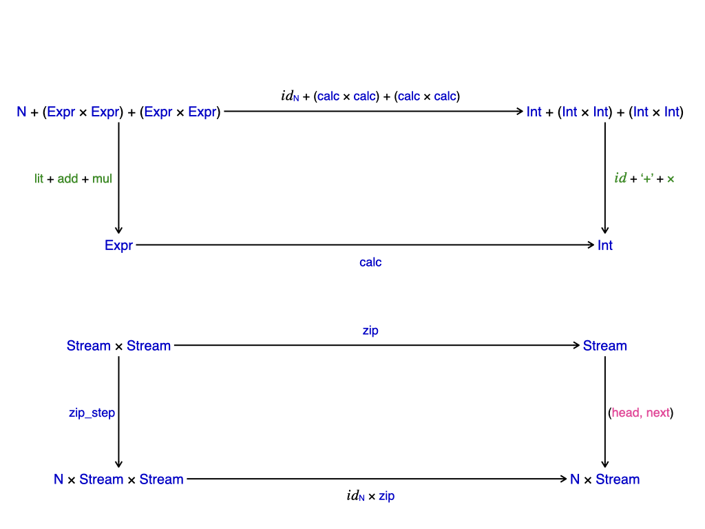
A -algebra homomorphism between two -algebras is any function where . Dually, an -coalgebra homomorphism between two -algebras is any function where . In terms of commuting diagrams these conditions amount to:

Once again, we’ve already seen examples of both algebra and coalgebra homomorphisms:
- is an -algebra homomorphism.
- is an -coalgebra homomorphism.
We leave it to the reader to check the commutativity conditions for these homomorphisms, which are summarised in the diagrams below:
The function above is defined as . If we keep use zipStep according to the (pseudo)-agda style code below we can recover the behaviour of .
So is in a sense equivalent to a single step of the function. This is not a coincidence! We’ll return to this point shortly when we talk about coinduction.
-algebras and algebra homomorphisms form a category. We refer to an initial object of this category as an initial algebra. Dually, -coalgebras and coalgebra homomorphisms form a category whose final objects we refer to as final coalgebras. Initiality and finality occupy a central role in universal (co)algebra. This is what we explore next.
Take an initial -algebra together with an arbitrary -algebra . By initiality, there exists a unique -algebra homomorphism . We say that such a function is inductively defined. Intuitively, an inductive function breaks complicated elements of down into their constituent parts, applies some function on each constituent part, and mixes the results together to obtain an action on the whole element. If you’re an eagle eyed reader you’ll know that we’ve already encountered a function that behaves this way. Remember how breaks complicated s down into smaller sub-s and mixes their results together to get a result for the whole ? Well now we know that this behaviour is indicative of the fact that is inductively defined (note that in this case is an initial -algebra3).
Now consider the dual scenario where we have a final -coalgebra together with an arbitrary -coalgebra . By universality there must be a unique coalgebra homomorphism . We call such a function g coinductively defined. A nice intuition here is to think of as a dynamic system evolving according to the transition structure given by , then the function is the result of applying the transition over and over again. Repeated application of a transition structure might sound awfully familiar to you, as in fact it should. We were only just talking about how can be thought of as repeated applications of . Again, this is indicative of the fact that is a coinductive definition, and that is a final coalgebra.
With that our whirlwind tour comes to a close. We’ve seen how universal algebra gives us tools for exploring the structure of things, while universal coalgebra allows us to explore their behaviour. Together they gave us a way to rigorously analyse the duality between structure and behaviour. Earlier in the article we made the rather bold claim that this duality transcends the examples we’ve seen here and goes up all the way to the foundations of thought. We’ll end on a similarly dramatic note by giving you a philosophical question to ponder:
Is a “thing” best defined by its constituent parts (structure) or by its observable actions(behaviour).
Further Reading
If you’re interested in learning more there’s many facets of the structure vs behaviour duality that we didn’t have space to talk about. Things like congruence vs bisimulation, minimality vs simplicity, and freeness vs cofreeness. A good starting point for further reading is the paper which motivated this blog post, Universal Coalgebra: a theory of systems. In this classic work the author introduces universal coalgebra as an abstract theory for capturing the behaviour of a wide class of dynamic systems4. Even though it is a fantastic introduction to universal coalgebra the focus on duality in this article is arguably limited. A paper that does extensively cover duality is An introduction to (co)algebra and (co)induction. This is also a great article for readers who may be newer to category theory as the material is presented in set-theoretic language whenever possible. Much of the material from both these papers is now available as part of an introductory book on coalgebras. Finally, since our examples focused on functional programming we mention that chapter 24 of Category Theory for Programmers gives a nice account of how (co)algebras are used in the functional programming language Haskell.
1 Agda is a functional programming language often used as a theorem prover. ↩
2 This definition can easily be generalised to endofunctors on an arbitrary category .↩
3 Proving this fact directly is a rather fun excercise that we leave for the reader. Hint: First build up a homomorphism from into an arbitrary -algebra by considering where could send elements such as 0 or add ( 5) ( ( 4) ( 2)) to in the target set. Then assume for the sake of contradiction that is not unique, i.e. send some of the objects to a different place in the target set. You should be able to show that this new function breaks the algebra homomorphism commutativity conditions. Once you’ve proven this have a go at showing that is a final coalgebra.↩
4 These so-called dynamic systems are by no means limited to the functional programming examples in this blog post. In fact, the main appeal of universal coalgebra comes from the omni-presence of dynamic systems around us. Labelled transition systems, finite automata, Kripke models arising in modal logic, And even the evolution of quantum systems are just a few examples of such systems.↩
Re: Structure vs. Observation
I already knew about datatype constructors, but I love the idea of datatype destructors. I now imagine that it’s part of a dual theory to constructive mathematics, called destructive mathematics. To be able to proclaim “I am a destructive mathematician” possibly even beats “I am a persistent homologist”.
(Sorry for the non-serious comment… I hope I’m not setting a precedent. BTW, the link to Amin’s web page doesn’t work.)