Native Type Theory (Part 3)
Posted by John Baez
.")
guest post by Christian Williams
We are continuing Native Type Theory. We described higher-order algebraic theories, categories with products and finite-order exponents, which present languages with (binding) operations, equations, and rewrites; from these we construct native type systems.
Now we use the wisdom of the Yoneda embedding.
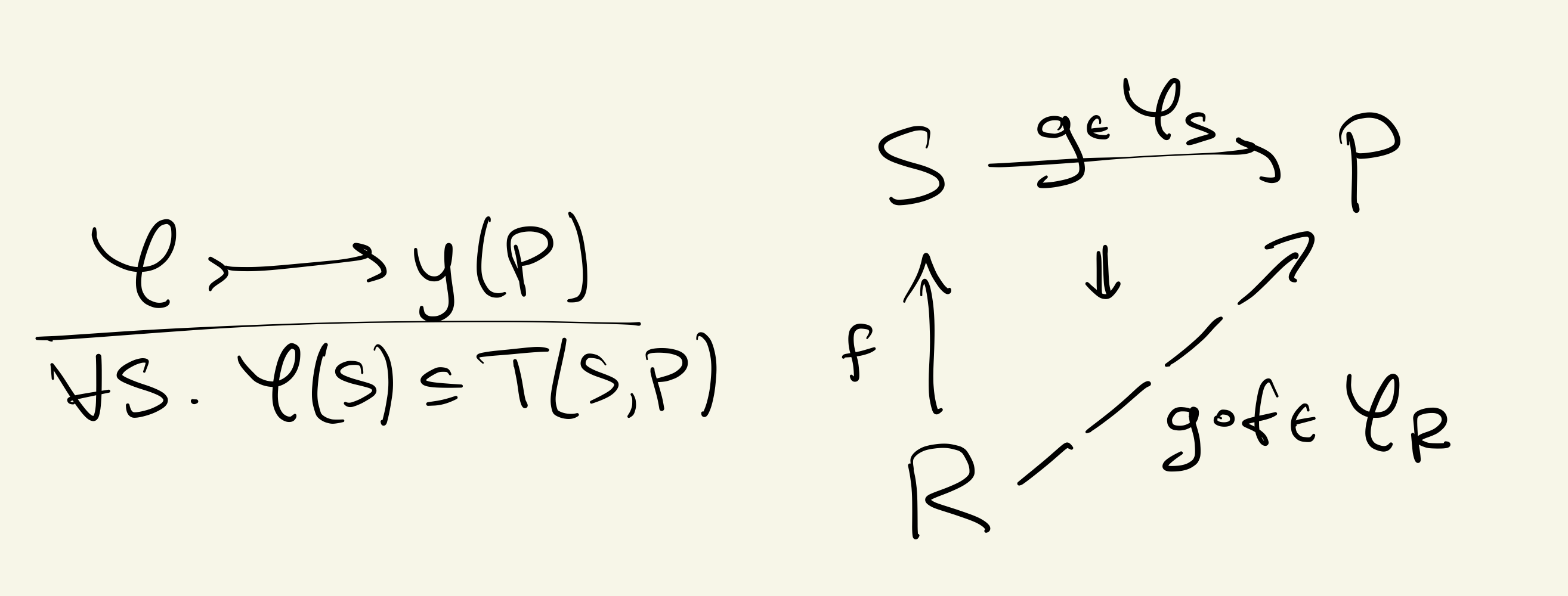
Every category embeds into a topos of presheaves
If is monoidal closed, then the embedding preserves this structure:
i.e. using Day convolution, is monoidal closed. So, we can move into a richer environment while preserving higher-order algebraic structure, or languages.
We now explore the native type system of a language, using the -calculus as our running example. The complete type system is in the paper, page 9.
Representables
The simplest kind of object of the native type system is a representable . This is the set of all terms of sort , indexed by the context of the language. Whereas many works in computer science either restrict to closed terms or lump all terms together, this indexing is natural and useful.
In the -calculus, is the indexed set of all processes.
The type system is built from these basic objects by the operations of and the structure of . We can then construct predicates, dependent types, co/limits, etc., and each constructor has corresponding inference rules which can be used by a computer.
Predicates and Types
The language of a topos is represented by two fibrations: the subobject fibration gives predicate logic, and the codomain fibration gives dependent type theory. Hence the two basic entities are predicates and (dependent) types. Types are more general, and we can think of them as the “new sorts” of language , which can be much more expressive.
.png)
A predicate corresponds to a subobject of a representable , which is equivalent to a sieve: a set of morphisms into , closed under precomposition:
This emphasizes the idea that predicate logic over representables is actually reasoning about abstract syntax trees: here is some tree of operations in with an -shaped hole of variables, and the predicate only cares about the outer shape of ; you can plug in any term while still satisfying .
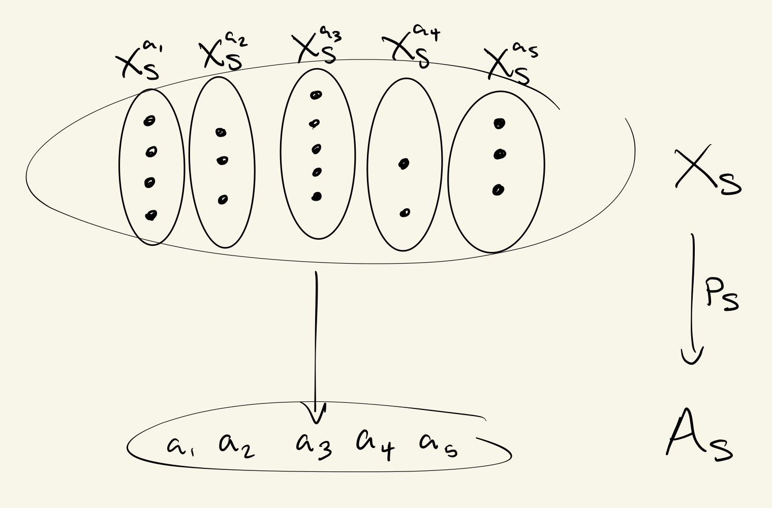
More generally, a morphism is understood as an “indexed presheaf” or dependent type
i.e. for every element , there is a fiber which is the “type depending on term ”.
An example of a type in the -calculus is given by the input operation,
where the fiber over is the set of all channel-context pairs such that .
Dependent Sum and Product
Here we use the structure described in Part I. The predicate functor is a hyperdoctrine, which for each presheaf gives a complete Heyting algebra of predicates , and for each gives adjoints for image, preimage, and secure image.
Similarly, the slice functor is a hyperdoctrine into co/complete toposes with adjoints . These are dependent sum, substitution, and dependent product. From these we can reconstruct all the operations of predicate logic, and much more.
As (briefly) explained in Part I, the idea of dependent sum is that indexed sums generalize products; here the codomain is the set of indices and its fibers are the sets in the family; so an element of the indexed sum is a dependent pair . Dually, indexed products generalize functions: an element of the product of the fibers is a tuple which can be understood as a dependent function where the codomain depends on which you plug in.
Explicitly, given and , , we have and
(letting and denote the fiber over ). Despite the complex formulae, the intuition is essentially the same as in Set, except we need to ensure the resulting objects are still presheaves, i.e. closed under precomposition. The point is:
The main examples start with just “pushing forward” operations in the theory, using . Given an operation , the image takes a predicate (sieve) and simply postcomposes every term in with .
Hence an example predicate (leaving and implicit) is
This predicate determines processes which are the parallel of two non-null processes.
As an example of the distinct utility of the adjoints, recall from Part 2 that we can model computational dynamics using a graph of processes and rewrites . Now these operations give adjunctions between sieves on and sieves on , which give operators for “step forward or backward”:
While “image” step-forward gives all possible next terms, the “secure” step-forward gives terms which could only have come from . For security protocols, this can be used to filter processes by past behavior.
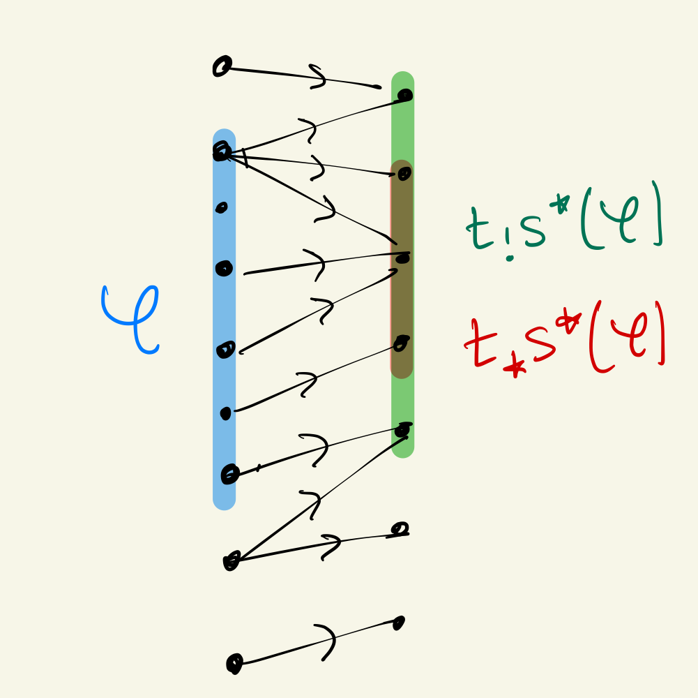
Image / Comprehension and Subtyping
Predicates and types are related by an adjunction between the fibrations.
To convert a predicate to a type, apply comprehension to construct the subobject of terms which satisfy . To convert a type to a predicate, apply image factorization to construct the predicate for whether each fiber is inhabited.
We implicitly use the comprehension direction all the time (thinking of predicates as their subobjects); and while taking the image is more destructive, it can certainly be useful for the sake of simplification. For example, rather than thinking about the type , we may simply want to consider the image , the set of all output processes.
Internal Hom and Reification
While the Grothendieck construction is relatively known, there is less awareness about how the local structure of an indexed category (complete Heyting algebras for predicates) can often be converted to a global structure on the total category of the corresponding fibration. The total category of the predicate functor is cartesian closed, allowing us to construct predicate homs.
The construction can be understood in the category of sets. Given and , we can define
Hence it constructs “contexts which ensure implications”.
For example, we can construct the “wand” of separation logic: let be the theory of a commutative monoid , with a set of constants adjoined as the elements of a heap. If we define
then asserts that .
There is a much more expressive way of forming homs which we call reification (p7); we do not know if it has been explored, and we have yet to determine its relation to dependent product.
co/Induction
Similarly, the fibers of are co/complete, and this can be assembled into a global co/complete structure on the total category. Hence, we can use this to construct co/inductive types.
For example, given a predicate on names , we may construct a predicate for “liveness and safety” on :
where denotes the initial algebra, which is constructed as a colimit. This determines whether a process inputs on , does not input on , and continues as a process which satisfies this same predicate. This can be understood as a static type for a firewall.
Applications
Once these type constructors are combined, they can express highly useful and complex ideas about code. The best part is that this type system can be generated from any language with product and function types, which includes large chunks of many popular programming languages.
To get a feel for more applications, check out the final section of Native Type Theory. Of course, check out the rest of the paper, and let me know what you think! Thank you for reading.