The n-Category Café

First, the bioctonionic plane is one of the four Rosenfeld planes:

• the octonionic projective plane $\mathbb{O}\text{P}^2$, a 16-dimensional compact Riemannian manifold on which the compact Lie group $\text{F}_4$ acts transitively as isometries, with the stabilizer of any point being $\text{Spin}(9)$. This is a symmetric space, and as such it’s called FII in Cartan’s classification.

• the bioctonionic plane $(\mathbb{C} \otimes \mathbb{O})\mathbb{P}^2$, a 32-dimensional compact Riemannian manifold on which the compact Lie group $\text{E}_6$ acts transitively as isometries, with the stabilizer of any point being $(\text{Spin}(10) \times \text{U}(1))/\mathbb{Z}_4$. This is the symmetric space EIII.

• the quateroctonionic plane $(\mathbb{H} \otimes \mathbb{O}) \mathbb{P}^2$, a 64-dimensional compact Riemannian manifold on which the compact Lie group $\text{E}_7$ acts transitively as isometries, with the stabilizer of any point being $(\text{Spin}(12) \times \text{Sp}(1))/\mathbb{Z}_2$. This is the symmetric space EVI.

• the octooctonionic plane $(\mathbb{O} \otimes \mathbb{O}) \mathbb{P}^2$, a 128-dimensional compact Riemannian manifold on which the compact Lie group $\text{E}_8$ acts transitively as isometries, with the stabilizer of any point being $\text{Spin}(16)/\mathbb{Z}_2$. This is the symmetric space EVIII.

There’s a nice network of systematic approaches to these spaces: they form one row of the so-called magic square, so one way to learn about the bioctonionic plane is to study the magic square, for example here:

• Chris H. Barton and Anthony Sudbery, Magic squares of Lie algebras. Available as arXiv:math/0001083; see also arXiv:0203010 for a “streamlined and extended” version, which has more yet also less.

Here you can also find lots of references to earlier work, e.g. to Freudenthal and Tits. The basic idea of the magic square is that you start with two normed division algebras $\mathbb{K}, \mathbb{K}'$ and from them you build a Lie algebra, which gives a Lie group $G(\mathbb{K},\mathbb{K}')$. There’s also a way to get a subgroup $H(\mathbb{K}, \mathbb{K}')$, and the quotient space

$$(\mathbb{K} \otimes \mathbb{K}')\text{P}^2 = G(\mathbb{K},\mathbb{K}')/H(\mathbb{K}, \mathbb{K}')$$

is a kind of ‘plane’ on which the group $G(\mathbb{K},\mathbb{K}')$ acts. If you take $\mathbb{K}' = \mathbb{O}$, this construction gives you the four Rosenfeld planes listed above.

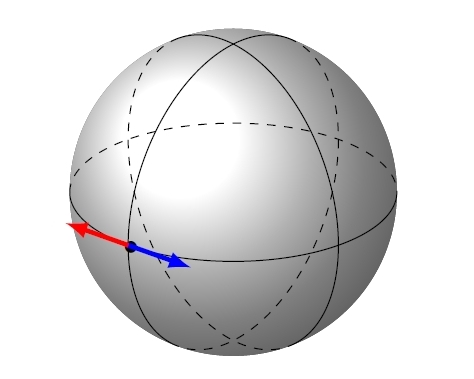
Each one of these planes is a compact Riemannian symmetric space: this means it’s a connected compact Riemannian manifold $M$ such that for each point $p \in M$ there’s an isometry

$$\sigma_p \colon M \to M$$

that fixes $p$, acts as $-1$ on its tangent space, and squares to the identity. This map is called ‘reflection across $p$’ for the obvious reason. For example, a round 2-sphere is a symmetric space, with the differential of $\sigma_p$ switching the red and blue tangent vectors:

Cartan classified compact Riemannian symmetric spaces, and there’s a nice theory of them. Any compact simple Lie group is one, and most of the rest come in infinite series connected to real and complex Clifford algebras, as I explained here. But there are 9 extra ones, all related to the octonions and exceptional Lie groups. The Rosenfeld planes are four of these.

You can learn this material starting on Wikipedia and then going to a textbook, ideally this:

• Sigurdur Helgason, Differential Geometry, Lie Groups and Symmetric Spaces, Academic Press, 1978.

Helgason taught me Lie theory when I was a grad student at MIT, so I have a fondness for his book—but it’s also widely accepted as the most solid text on symmetric spaces!

The bioctonionic plane is even better: it’s a compact hermitian symmetric space: a compact Riemannian symmetric space $M$ where each tangent space $T_p M$ has a complex structure

$$J \colon T_p M \to T_p M , \qquad J^2 = -1$$

compatible with the metric, and reflection about each point preserves this complex structure. I mentioned that the bioctonionic plane is

$$(\mathbb{C} \otimes \mathbb{O})\text{P}^2 \cong G(\mathbb{C},\mathbb{O})/H(\mathbb{C},\mathbb{O})$$

where

$$G(\mathbb{C},\mathbb{O}) = \text{E}_6$$

acts transitively, and the stabilizer of a point is

$$H(\mathbb{C}, \mathbb{O}) = (\text{Spin}(10) \times \text{U}(1))/\mathbb{Z}_4$$

The $\text{U}(1)$ here comes from the complex structure!

Wikipedia is especially thorough on hermitian symmetric spaces, so if you want to delve into those, start here:

• Wikipedia, Hermitian symmetric space.

Another tack is to focus on the exceptional Lie groups $\text{F}_4, \text{E}_6, \text{E}_7$ and $\text{E}_8$ and their connection to the nonassociative algebras $\mathfrak{h}_3(\mathbb{O})$, $\mathfrak{h}_3(\mathbb{C} \otimes \mathbb{O})$, $\mathfrak{h}_3(\mathbb{H} \otimes \mathbb{O})$ and $\mathfrak{h}_3(\mathbb{O} \otimes \mathbb{O})$, respectively. Here I recommend this:

• Ichiro Yokota, Exceptional Lie Groups. Available as arXiv:0902.0431. (See especially Chapter 3, for $\text{E}_6$ and the complexified exceptional Jordan algebra $\mathfrak{h}_3(\mathbb{C} \otimes \mathbb{O})$.)

If you have a fondness for algebra you may also want to learn how symmetric spaces arise from Jordan triple systems or Jordan pairs. This is important if we wish to see the bioctonionic plane as the space of pure states of some exotic quantum system!

Now, this is much easier to do for the octonionic plane, because that’s the space of pure states for the exceptional Jordan algebra $\mathfrak{h}_3(\mathbb{O})$, which is a Euclidean Jordan algebra, meaning one in which a sum of squares can only be zero if all those squares are zero. You can think of a Euclidean algebra $A$ as consisting of observables, with the sums of squares being ‘nonnegative’ observables. These nonnegative observables form a convex cone $K \subseteq A$. The dual vector space $A^\ast$ contains a cone of linear functionals $f$ that send these nonnegative observables to nonnegative real numbers — I’ll call this the dual cone $K^\ast$. The functionals $f \in K^\ast$ with $f(1) = 1$ are called states. The states form a convex set, and the extreme points are called pure states. All of this fits nicely into a modern framework for understanding quantum theory and potential generalizations, called ‘generalized probabilistic theories’:

• Howard Barnum, Alexander Wilce, Post-classical probability theory, in Quantum Theory: Informational Foundations and Foils, eds. Giulio Chiribella, Robert W. Spekkens, Springer, 2016. (See Section 5 for Jordan algebras, and ignore the fact that they say the exceptional Jordan algebra consists of $2 \times 2$ matrices: they know perfectly well that they’re $3 \times 3$.)

The underlying math, with a lot more about symmetric spaces, cones and Euclidean Jordan algebras but with none of the physics interpretation, is wonderfully explained here:

• Jacques Faraut and Adam Korányi, Analysis on Symmetric Cones, Oxford U. Press, 1994.

A crucial fact throughout this book is that when you start with a Euclidean Jordan algebra $A$, its cone $K$ of nonnegative observables is self-dual: there’s an isomorphism of vector spaces $A \cong A^\ast$ that maps $K$ to $K^\ast$ in a one-to-one and onto way. The cone $K$ is also homogeneous, meaning that the group of invertible linear transformations of $A$ preserving $K$ acts transitively on the interior of $K$. Faraut and Kor´nyi call a self-dual homogeneous cone a symmetric cone — and they show that any symmetric cone comes from a Euclidean Jordan algebra! This result plays an important role in modern work on the foundations of quantum theory.

Unfortunately, I’m telling you all this nice stuff about Euclidean Jordan algebras and symmetric cones just to say that while all this applies to the octonionic projective plane, sadly, it does not apply to the bioctonionic plane! The bioctonionic plane does not come from a Euclidean Jordan algebra or a symmetric cone. Thus, to understand it as a space of pure states, we’d have to resort to a more general formalism.

There are a few papers that attempt exactly this:

• Lawrence C. Biedenharn and Piero Truini, An $\mathcal{E}_6 \otimes \mathcal{U}(1)$ invariant quantum mechanics for a Jordan pair, Journal of Mathematical Physics 23 (1982), 1327-1345.

• Lawrence C. Biedenharn and Piero Truini, Exceptional groups and elementary particle structures, Physica A: Statistical Mechanics and its Applications 14 (1982), 257–270.

• Lawrence C. Biedenharn, G. Olivieri and Piero Truini, Three graded exceptional algebras and symmetric spaces, Zeitschrift Physik C — Particles and Fields 33 (1986), 47–65.

Here’s the basic idea. We can define $\mathfrak{h}_3(\mathbb{C} \otimes \mathbb{O})$ to consist of $3 \times 3$ hermitian matrices with entries in $\mathbb{C} \otimes \mathbb{O}$, where ‘hermitian’ is defined using the star-algebra structure on $\mathbb{C} \otimes \mathbb{O}$ where we conjugate the octonion part but not the complex part! Then $\mathfrak{h}_3(\mathbb{C} \otimes \mathbb{O})$ is just the complexification of $\mathfrak{h}_3(\mathbb{O})$:

$$\mathfrak{h}_3(\mathbb{C} \otimes \mathbb{O}) \cong \mathbb{C} \otimes \mathfrak{h}_3(\mathbb{O})$$

Then because $\mathfrak{h}_3(\mathbb{O})$ is a Jordan algebra over $\mathbb{R}$, $\mathfrak{h}_3(\mathbb{C} \otimes \mathbb{O})$ is a Jordan algebra over $\mathbb{C}$. So we can do a lot with it. But it’s not a Euclidean Jordan algebra.

Puzzle. Show that it’s not.

So, Biedenharn and Truini need a different approach to relate $\mathfrak{h}_3(\mathbb{C} \otimes \mathbb{O})$ to some sort of exotic quantum system. And they use an approach already known to mathematicians: namely, the theory of Jordan pairs! Here you work, not with a single element of $\mathfrak{h}_3(\mathbb{C} \otimes \mathbb{O})$, but with a pair.

Jordan triple systems and Jordan pairs are two closely related generalizations of Jordan algebras. I’ve been working on the nLab articles about these concepts, so click the links if you want to learn more about them. I explain how either of these things gives you a 3-graded Lie algebra — that is, a $\mathbb{Z}$-graded Lie algebra that is nonvanishing only in the middle 3 grades:

$$\mathfrak{g} = \mathfrak{g}_{-1} \oplus \mathfrak{g}_0 \oplus \mathfrak{g}_1$$

And from a 3-graded Lie algebra you can get a symmetric space $G/H$ where the Lie algebra of $G$ is $\mathfrak{g}$ and the Lie algebra of $H$ is $\mathfrak{g}_0$. Each tangent space of this symmetric space is thus isomorphic to $\mathfrak{g}_{-1} \oplus \mathfrak{g}_1$.

In the case relevant to the bioctonionic plane, the 3-graded Lie algebra is

$$\mathfrak{e}_6 = (\mathbb{C} \otimes \mathbb{O}) \; \oplus \; (\mathfrak{so}(10) \oplus \mathbb{R}) \; \oplus \; (\mathbb{C} \otimes \mathbb{O})$$

So, the bioctonionic plane is a symmetric space on which $\text{E}_6$ acts, with stabilizer group $\text{Spin}(10) \times \text{U}(1)$ (up to covering spaces), and with tangent space isomorphic to $(\mathbb{C} \otimes \mathbb{O})^2$.

So all this is potentially very nice. For much more on this theory, try the work of Ottmar Loos:

• Ottmar Loos, Symmetric Spaces, Volume 1: General Theory, W. A. Benjamin, 1969.

• Ottmar Loos, Symmetric Spaces, Volume 2: Compact Spaces and Classification, W. A. Benjamin, 1969.

• Ottmar Loos, Jordan Pairs, Lecture Notes in Mathematics 460, Springer, Berlin, 1975.

• Ottmar Loos, Jordan triple systems, $R$-spaces, and bounded symmetric domains, Bulletin of the American Mathematical Society 77 (1971), 558–561.

• Ottmar Loos, Bounded Symmetric Domains and Jordan Pairs, Mathematical Lectures, University of California, Irvine, 1977.

That’s a lot of stuff! For a quick overview of Loos’ work, I find this helpful:

• Kevin McCrimmon, Jordan Pairs, by Ottmar Loos, review in Bulletin of the American Mathematical Society 84 4 (1978), 685–690.

Unfortunately Loos does not delve into examples, particularly the bioctonionic plane. For that, try Biedenharn and Truini, and also these:

• Daniele Corradetti, Alessio Marrani, David Chester and R. Aschheim, Conjugation matters: bioctonionic Veronese vectors and Cayley-Rosenfeld planes, Int. J. Geom. Meth. Mod. Phys. 19 (2022), 2250142.

• Jian Qiu, Plücker coordinates and the Rosenfeld planes, Journal of Geometry and Physics 206 (2024), 105331.

• Latham Boyle, The Standard Model, the exceptional Jordan algebra, and triality.

This last one is what got me interested in this subject in the first place! Latham Boyle works at the University of Edinburgh, and being able to talk to someone who understands octonions and physics so well is very energizing.

I should devote a whole article to Latham’s paper sometime — and in particular, why the bioctonionic plane may be better than the octonionic projective plane for particle physics. But the short answer is that tangent space of any point of the bioctonionic plane is a copy of $(\mathbb{C} \otimes \mathbb{O})^2$, a 16-dimensional complex vector space. Sitting in the stabilizer group of this point is a copy of $\text{Spin}(10)$, and sitting in there is a copy of the Standard Model gauge group! And that group acts on $(\mathbb{C} \otimes \mathbb{O})^2$ just like it does on one generation of fermions (not their antiparticles). If we try the same trick using the octonionic projective plane, we still get the Standard Model gauge group, but its action on the tangent space is its action only on left-handed fermions.

To wrap things up, I should say a bit about ‘Hjelmslev planes’, since the bioctonionic plane is supposed to be one of these. Axiomatically, a Hjelmslev plane is a set $P$ of points, a set $L$ of lines, and an incidence relation between points and lines. We require that for any two distinct points there is at least one line incident to both, and for any two distinct line there is at least one point incident to both. If two points are incident to more than one line we say they are neighbors. If two lines are incident to more than one point we say they are neighbors. We demand that both these ‘neighbor’ relations are equivalence relations, and that if we quotient $P$ and $L$ by these equivalence relations, we get an axiomatic projective plane.

Challenge. What projective plane do we get if we apply this quotient construction to the bioctonionic plane?

My only guess is that we get the octonionic projective plane — but I don’t know why.

The literature on Hjelmslev planes seems a bit difficult, but I’m finding this to be a good introduction:

• Joanne L. Hall and Asha Rao, An algorithm for constructing Hjelmslev planes, in Algebraic Design Theory and Hadamard Matrices, Springer, 2014.

The answer to my puzzle should be here, because they’re talking about Hjelmslev planes built using split octonion algebras (like $\mathbb{C} \otimes \mathbb{O}$):

• Tonny A. Springer and Ferdinand D. Veldkamp, On Hjelmslev–Moufang planes, Mathematicsche Zeitschrift 107 (1968), 249–263.

But I don’t see the answer here yet!