Skip to the Main Content

Note:These pages make extensive use of the latest XHTML and CSS Standards. They ought to look great in any standards-compliant modern browser. Unfortunately, they will probably look horrible in older browsers, like Netscape 4.x and IE 4.x. Moreover, many posts use MathML, which is, currently only supported in Mozilla. My best suggestion (and you will thank me when surfing an ever-increasing number of sites on the web which have been crafted to use the new standards) is to upgrade to the latest version of your browser. If that's not possible, consider moving to the Standards-compliant and open-source Mozilla browser.

November 10, 2020

Octonions and the Standard Model (Part 8)

Posted by John Baez

Last time I described the symmetry group E 6\mathrm{E}_6 of the exceptional Jordan algebra in terms of 10d Minkowski spacetime. We saw that in some sense it consists of four parts:

  • the double cover of the Lorentz group in 10 dimensions,
  • translations in left-handed spinor directions,
  • translations in right-handed spinor directions, and
  • ‘dilations’ (rescalings).

But our treatment was computational: the geometrical meaning of this decomposition was left obscure. As Atiyah said:

Algebra is the offer made by the devil to the mathematician. The devil says: I will give you this powerful machine, it will answer any question you like. All you need to do is give me your soul: give up geometry and you will have this marvellous machine.

Now let’s renounce the devil’s bargain and try to understand the geometry! Jordan algebras are deeply connected to projective geometry, and the exceptional Jordan algebra is all about the octonionic projective plane.

Let’s start with a baby example: instead of the exceptional Jordan algebra of 3×33 \times 3 self-adjoint octonionic matrices, 𝔥 3(𝕆)\mathfrak{h}_3(\mathbb{O}), let’s look at the Jordan algebra of 2×22 \times 2 self-adjoint complex matrices:

𝔥 2()={(t+z xiy x+iy tz):t,x,y,z} \mathfrak{h}_2(\mathbb{C}) = \left\{ \left( \begin{array}{cc} t+z & x- i y \\ x+ i y & t-z \end{array} \right) : \; t,x,y,z \in \mathbb{R} \right\}

The determinant makes this into a copy of 4d Minkowski spacetime:

det(t+z xiy x+iy tz)=t 2x 2y 2z 2 \mathrm{det} \left( \begin{array}{cc} t+z & x - i y \\ x + i y & t-z \end{array} \right) = t^2 - x^2 - y^2 - z^2

Any nonzero self-adjoint matrix with determinant zero spans a ‘light ray’ — a line through the origin in Minkowski spacetime that describes the path of something moving at the speed of light.

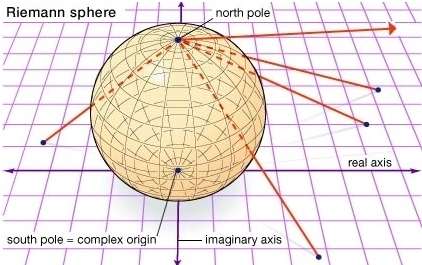
If you stand at the origin of 4d Minkowski spacetime — which in fact is exactly where you are — the set of light rays passing through you form a 2-sphere. This is the sphere of things you could see if you could freely turn your head in every direction. It’s often called the ‘heavenly sphere’, since it’s the starry sky surrounding you when you’re floating in outer space.

As you turn your head your view gets rotated — and if you’re moving, your view is Lorentz transformed, with the stars in front of you bunching up, though this effect is only noticeable if you’re moving at close to the speed of light. So, special relativity gives an action of the Lorentz group SO(3,1)SO(3,1) on the heavenly sphere.

But the heavenly sphere is a copy of the Riemann sphere, P 1\mathbb{C}\mathrm{P}^1 — and the identity component of the Lorentz group acts as conformal transformations of P 1\mathbb{C}\mathrm{P}^1. These transformations form the group PSL(2,)\mathrm{PSL}(2,\mathbb{C}). So, we get an isomorphism

PSL(2,)SO 0(3,1) \mathrm{PSL}(2,\mathbb{C}) \cong \mathrm{SO}_0(3,1)

We can see this in more detail as follows. As I’ve mentioned, any nonzero matrix in 𝔥 2()\mathfrak{h}_2(\mathbb{C}) with determinant zero yields a light ray through the origin. But any nonzero vector ψ 2\psi \in \mathbb{C}^2 gives such a matrix:

p=ψψ 𝔥 2() p = \psi \psi^\dagger \in \mathfrak{h}_2(\mathbb{C})

So it gives such a light ray! Indeed, we get all such light rays in this manner. But multiplying ψ\psi by an invertible complex number just rescales pp, so it doesn’t change the light ray. So the set of light rays through the origin is P 1\mathbb{C}\mathrm{P}^1.

Pursuing this further, we can see how SL(2,)\mathrm{SL}(2,\mathbb{C}) acts on nonzero vectors ψ 2\psi \in \mathbb{C}^2, and thus PSL(2,)\mathrm{PSL}(2,\mathbb{C}) acts on the heavenly sphere P 1\mathbb{C}\mathrm{P}^1.

Now, let us use these ideas to break the group PSL(2,)\mathrm{PSL}(2,\mathbb{C}) into four pieces, analogous to the four pieces of E 6\mathrm{E}_6 that we worked out last time. This is not hard.

The heavenly sphere P 1\mathbb{C}\mathrm{P}^1 can be seen as \mathbb{C} together with a point at infinity:

Then:

  • Rotations about the origin in \mathbb{C} form a subgroup of PSL(2,)\mathrm{PSL}(2,\mathbb{C}) isomorphic to SO(2)\mathrm{SO}(2). These transformations preserve the origin and the point at infinity.

  • Translations in \mathbb{C} form an abelian subgroup of PSL(2,)\mathrm{PSL}(2,\mathbb{C}) isomorphic to \mathbb{C}. These transformations preserve the point at infinity.

  • The point at infinity is the origin of an ‘antipodal’ copy of \mathbb{C} in the heavenly sphere, and translations in this copy of \mathbb{C} form another abelian subgroup of PSL(2,)\mathrm{PSL}(2,\mathbb{C}), also isomorphic to \mathbb{C}. These transformations preserve the origin.

  • Dilations of the original copy of \mathbb{C} also act as dilations of the antipodal copy of \mathbb{C}. These form an abelian subgroup isomorphic to \mathbb{R}. These transformations preserve the origin and the point at infinity.

At the Lie algebra level this gives

𝔰𝔬(3,1)𝔰𝔬(2) \mathfrak{so}(3,1) \cong \mathfrak{so}(2) \oplus \mathbb{C} \oplus \mathbb{C} \oplus \mathbb{R}

This is an isomorphism of vector spaces, not of Lie algebras: the four parts are Lie subalgebras, but they don’t commute with each other!

I believe that this is beautifully analogous to what we saw last time:

𝔢 6𝔰𝔬(9,1)𝕆 2𝕆 2 \mathfrak{e}_6 \cong \mathfrak{so}(9,1) \oplus \mathbb{O}^2 \oplus \mathbb{O}^2 \oplus \mathbb{R}

where again the four parts are Lie subalgebras that don’t commute with each other. This fancier version differs in two ways: we are replacing the complex numbers with the octonions, and we are replacing a 2d story with a 3d story.

Just as the group PSL(2,)\mathrm{PSL}(2,\mathbb{C}) acts on P 1\mathbb{C}\mathrm{P}^1, the group E 6\mathrm{E}_6 acts on 𝕆P 2\mathbb{O}\mathrm{P}^2. Just as P 1\mathbb{C}\mathrm{P}^1 consists of \mathbb{C} together with a point at infinity, 𝕆P 2\mathbb{O}\mathrm{P}^2 consists of 𝕆 2\mathbb{O}^2 together with a ‘line at infinity’. And this let us break E 6\mathrm{E}_6 into four parts:

  • There is a Spin(9,1)\mathrm{Spin}(9,1) subgroup of E 6\mathrm{E}_6 acting as linear transformations of 𝕆 2𝕆P 2\mathbb{O}^2 \subseteq \mathbb{O} \mathrm{P}^2. These preserve both the origin and the line at infinity.

  • Translations of 𝕆 2\mathbb{O}^2 form an abelian subgroup of E 6\mathrm{E}_6 isomorphic to 𝕆 2\mathbb{O}^2. These preserve the line at infinity.

  • The space of lines in 𝕆P 2\mathbb{O} \mathrm{P}^2 form a ‘dual’ copy of 𝕆P 2\mathbb{O} \mathrm{P}^2. Lines that miss the origin form a copy of 𝕆 2\mathbb{O}^2 in this dual 𝕆P 2\mathbb{O} \mathrm{P}^2. Translations of this other 𝕆 2\mathbb{O}^2 form another abelian subgroup of E 6\mathrm{E}_6 isomorphic to 𝕆 2\mathbb{O}^2. These preserve the origin.

  • Dilations, i.e. rescalings of 𝕆 2\mathbb{O}^2, form an abelian subgroup isomorphic to \mathbb{R}. These preserve both the origin and the line at infinity.

I need to confirm that this geometrical picture is really correct, and matches the algebraic story from last time. To match that story, one copy of 𝕆 2\mathbb{O}^2 should transform in the left-handed spinor representation of Spin(9,1)\mathrm{Spin}(9,1), while the other should transform in the right-handed spinor representation. Since the dilations commute with Spin(9,1)\mathrm{Spin}(9,1), their Lie algebra transforms in the trivial 1-dimensional representation of Spin(9,1)\mathrm{Spin}(9,1), as it should: this is the ‘scalar’ representation.

I will say more about this next time.

To flesh out the picture, it’s also important to compare two other Jordan algebras: 𝔥 2(𝕆)\mathfrak{h}_2(\mathbb{O}) and 𝔥 3()\mathfrak{h}_3(\mathbb{C}). Both these contain 𝔥 2()\mathfrak{h}_2(\mathbb{C}) and sit inside 𝔥 3(𝕆)\mathfrak{h}_3(\mathbb{O}). And both play a role in Dubois–Violette and Todorov’s description of the Standard Model gauge group, which we saw in Part 4. We met the first in Part 5: it’s 10-dimensional Minkowski spacetime! The second resembles the exceptional Jordan algebra, but without the complications arising from the octonions.

In fact we could also get the other division algebras into the act! We have Jordan algebra inclusions

𝔥 2() 𝔥 2() 𝔥 2() 𝔥 2(𝕆) 𝔥 3() 𝔥 3() 𝔥 3() 𝔥 3(𝕆) \begin{array}{ccccccc} \mathfrak{h}_2(\mathbb{R}) & \subset & \mathfrak{h}_2(\mathbb{C}) & \subset & \mathfrak{h}_2(\mathbb{H}) & \subset & \mathfrak{h}_2(\mathbb{O}) \\ \cap & & \cap & & \cap & & \cap \\ \mathfrak{h}_3(\mathbb{R}) & \subset & \mathfrak{h}_3(\mathbb{C}) & \subset & \mathfrak{h}_3(\mathbb{H}) & \subset & \mathfrak{h}_3(\mathbb{O}) \\ \end{array}

where the top four are 3d, 4d, 6d and 10d Minkowski spacetime, and the bottom four are ‘exotic spacetimes’ where the determinant vanishes on a light-cone described by a cubic equation instead of a quadratic one.

These Jordan algebra inclusions give inclusions of projective geometries:

P 1 P 1 P 1 𝕆P 1 P 2 P 2 P 2 𝕆P 2 \begin{array}{ccccccc} \mathbb{R}\mathrm{P}^1 & \subset & \mathbb{C}\mathrm{P}^1 & \subset & \mathbb{H}\mathrm{P}^1 & \subset & \mathbb{O}\mathrm{P}^1 \\ \cap & & \cap & & \cap & & \cap \\ \mathbb{R}\mathrm{P}^2 & \subset & \mathbb{C}\mathrm{P}^2 & \subset & \mathbb{H}\mathrm{P}^2 & \subset & \mathbb{O}\mathrm{P}^2 \end{array}

The top four are projective lines: the heavenly spheres in Minkowski spacetimes of dimensions 3, 4, 6 and 10. The bottom four are projective planes.

Each Jordan algebra has a determinant function, and a group of linear transformations preserving this determinant, so we also get these inclusions of Lie groups:

PSL(2,) PSL(2,) PSL(2,) PSL(2,𝕆) PSL(3,) PSL(3,) PSL(3,) PSL(3,𝕆) \begin{array}{ccccccc} \mathrm{PSL}(2,\mathbb{R}) & \subset & \mathrm{PSL}(2,\mathbb{C}) & \subset & \mathrm{PSL}(2,\mathbb{H}) & \subset & \mathrm{PSL}(2,\mathbb{O}) \\ \cap & & \cap & & \cap & & \cap \\ \mathrm{PSL}(3,\mathbb{R}) & \subset & \mathrm{PSL}(3,\mathbb{C}) & \subset & \mathrm{PSL}(3,\mathbb{H}) & \subset & \mathrm{PSL}(3,\mathbb{O}) \end{array}

Here the two row consists of Lorentz groups, or more precisely their identity components:

PSL(2,) SO 0(2,1) PSL(2,) SO 0(3,1) PSL(2,) SO 0(5,1) PSL(2,𝕆) SO 0(9,1) \begin{array}{ccl} \mathrm{PSL}(2,\mathbb{R}) & \cong & \mathrm{SO}_0(2,1) \\ \mathrm{PSL}(2,\mathbb{C}) & \cong & \mathrm{SO}_0(3,1) \\ \mathrm{PSL}(2,\mathbb{H}) & \cong & \mathrm{SO}_0(5,1) \\ \mathrm{PSL}(2,\mathbb{O}) & \cong & \mathrm{SO}_0(9,1) \end{array}

Defining PSL(2,𝕆)\mathrm{PSL}(2,\mathbb{O}) takes some work; I explained one approach here:

Defining PSL(3,𝕆)\mathrm{PSL}(3,\mathbb{O}) is even harder, so we might as well just come out and say it’s E 6\mathrm{E}_6, the group I’ve been talking about all along.

You may wonder where I’m going with all this. It would be easy to be seduced into endless explorations of all this math, and all the math it’s connected to, and all the math that is connected to… but I really have a specific goal in mind.

I’m trying to understand Dubois–Violette and Todorov’s description of the Standard Model gauge group in a more conceptual way. As we saw, this crucially involves picking a copy of \mathbb{C} inside 𝕆\mathbb{O}, and also a copy of 𝔥 2(𝕆)\mathfrak{h}_2(\mathbb{O}) inside 𝔥 3(𝕆)\mathfrak{h}_3(\mathbb{O}) — that is, 10d Minkowski spacetime inside the exceptional Jordan algebra.

This is why, out of this big diagram:

𝔥 2() 𝔥 2() 𝔥 2() 𝔥 2(𝕆) 𝔥 3() 𝔥 3() 𝔥 3() 𝔥 3(𝕆) \begin{array}{ccccccc} \mathfrak{h}_2(\mathbb{R}) & \subset & \mathfrak{h}_2(\mathbb{C}) & \subset & \mathfrak{h}_2(\mathbb{H}) & \subset & \mathfrak{h}_2(\mathbb{O}) \\ \cap & & \cap & & \cap & & \cap \\ \mathfrak{h}_3(\mathbb{R}) & \subset & \mathfrak{h}_3(\mathbb{C}) & \subset & \mathfrak{h}_3(\mathbb{H}) & \subset & \mathfrak{h}_3(\mathbb{O}) \\ \end{array}

I want to focus on this part:

𝔥 2() 𝔥 2(𝕆) 𝔥 3() 𝔥 3(𝕆) \begin{array}{ccccccc} \mathfrak{h}_2(\mathbb{C}) & \subset & \mathfrak{h}_2(\mathbb{O}) \\ \cap & & \cap \\ \mathfrak{h}_3(\mathbb{C}) & \subset & \mathfrak{h}_3(\mathbb{O}) \\ \end{array}

and its consequences.


  • Part 1. How to define octonion multiplication using complex scalars and vectors, much as quaternion multiplication can be defined using real scalars and vectors. This description requires singling out a specific unit imaginary octonion, and it shows that octonion multiplication is invariant under SU(3)\mathrm{SU}(3).
  • Part 2. A more polished way to think about octonion multiplication in terms of complex scalars and vectors, and a similar-looking way to describe it using the cross product in 7 dimensions.
  • Part 3. How a lepton and a quark fit together into an octonion — at least if we only consider them as representations of SU(3)\mathrm{SU}(3), the gauge group of the strong force. Proof that the symmetries of the octonions fixing an imaginary octonion form precisely the group SU(3)\mathrm{SU}(3).
  • Part 4. Introducing the exceptional Jordan algebra 𝔥 3(𝕆)\mathfrak{h}_3(\mathbb{O}): the 3×33 \times 3 self-adjoint octonionic matrices. A result of Dubois-Violette and Todorov: the symmetries of the exceptional Jordan algebra preserving their splitting into complex scalar and vector parts and preserving a copy of the 2×22 \times 2 adjoint octonionic matrices form precisely the Standard Model gauge group.
  • Part 5. How to think of 2×22 \times 2 self-adjoint octonionic matrices as vectors in 10d Minkowski spacetime, and pairs of octonions as left- or right-handed spinors.
  • Part 6. The linear transformations of the exceptional Jordan algebra that preserve the determinant form the exceptional Lie group E 6\mathrm{E}_6. How to compute this determinant in terms of 10-dimensional spacetime geometry: that is, scalars, vectors and left-handed spinors in 10d Minkowski spacetime.
  • Part 7. How to describe the Lie group E 6\mathrm{E}_6 using 10-dimensional spacetime geometry. This group is built from the double cover of the Lorentz group, left-handed and right-handed spinors, and scalars in 10d Minkowski spacetime.
  • Part 8. A geometrical way to see how E 6\mathrm{E}_6 is connected to 10d spacetime, based on the octonionic projective plane.
  • Part 9. Duality in projective plane geometry, and how it lets us break the Lie group E 6\mathrm{E}_6 into the Lorentz group, left-handed and right-handed spinors, and scalars in 10d Minkowski spacetime.
  • Part 10. Jordan algebras, their symmetry groups, their invariant structures — and how they connect quantum mechanics, special relativity and projective geometry.
Posted at November 10, 2020 8:43 PM UTC

TrackBack URL for this Entry:   https://golem.ph.utexas.edu/cgi-bin/MT-3.0/dxy-tb.fcgi/3263

11 Comments & 0 Trackbacks

Re: Octonions and the Standard Model (Part 8)

Indeed, didn’t Faust eventually use algebra to discover his true love? And by discovering geometry, he ascended to heaven?

So it seems that there is good precedence in first using algebra to find the answer, and then using geometry to understand the answer.

Posted by: Theo Johnson-Freyd on November 10, 2020 11:45 PM | Permalink | Reply to this

Re: Octonions and the Standard Model (Part 8)

Theo wrote:

Indeed, didn’t Faust eventually use algebra to discover his true love? And by discovering geometry, he ascended to heaven?

Embarassingly, I don’t actually know the story. How did this work?

One great thing about computation is that it’s a way to “let your pencil do the thinking”, leading you to insights not easily reached by mental pictures or verbal / conceptual reasoning.

Btw, it’s unfair to identify “algebra” with “computation”, since there’s a lot of verbal / conceptual reasoning in algebra, which is very different than computation: it proceeds via a chain of insights.

Posted by: John Baez on November 11, 2020 4:10 PM | Permalink | Reply to this

Re: Octonions and the Standard Model (Part 8)

𝕆 2\mathbb{O}^2 together with a ‘line at infinity’.

It’s worth mentioning that that line is a projective line, hence it is itself 𝕆\mathbb{O} plus another point.

PSL(2,𝕆)\mathrm{PSL}(2,\mathbb{O}) is even harder, so we might as well just come out and say it’s E 6\mathrm{E}_6

Do you mean PSL(3,𝕆)\mathrm{PSL}(3,\mathbb{O}) here?

Posted by: David Roberts on November 11, 2020 12:11 AM | Permalink | Reply to this

Re: Octonions and the Standard Model (Part 8)

Yes, I meant PSL(3,𝕆)PSL(3,\mathbb{O}). Thanks, I’ll fix that.

And yes, the line at infinity in a projective plane is a projective line. This is one reason it’s helpful to think hard about 𝕆P 1\mathbb{O}\mathrm{P}^1 if you’re interested in 𝕆P 2\mathbb{O}\mathrm{P}^2. The ‘heavenly sphere’ in the exceptional Jordan algebra — the set of light rays through the origin — is not really a sphere but 𝕆P 2\mathbb{O}\mathrm{P}^2. But this is 𝕆 2\mathbb{O}^2 together with a copy of 𝕆P 1\mathbb{O}\mathrm{P}^1, which is the heavenly sphere in 10d Minkowski spacetime!

So there’s a small sky in the big sky. The symmetry group of the big sky is E 6\mathrm{E}_6, but the subgroup preserving the small sky is Spin(9,1)Spin(9,1)

Posted by: John Baez on November 11, 2020 2:25 AM | Permalink | Reply to this

Re: Octonions and the Standard Model (Part 8)

At the nnLab we have that E6 may be written as SL(3,𝕆)SL(3, \mathbb{O}). What difference does the ‘P’ make?

Posted by: David Corfield on November 11, 2020 4:36 PM | Permalink | Reply to this

Re: Octonions and the Standard Model (Part 8)

David wrote:

At the nnLab we have that E6 may be written as SL(3,𝕆)SL(3, \mathbb{O}). What difference does the ‘P’ make?

The short answer is: none.

The long answer is:

SL(3,𝕆)SL(3, \mathbb{O}) is a somewhat mystical entity: there’s no group of invertible 3×33 \times 3 octonionic matrices to be GL(3,𝕆)GL(3, \mathbb{O}), since octonion multiplication is nonassociative, and there’s no good concept of the determinant of a 3×33 \times 3 octonionic matrix — at least that I know of — to pick out a subgroup SL(3,𝕆)SL(3, \mathbb{O}).

If we could get over these roadbumps, we might define PSL(3,𝕆)PSL(3, \mathbb{O}) to be SL(3,𝕆)SL(3, \mathbb{O}) modulo its center. But it turns out that E 6E_6 has trivial center, so if we declare that SL(3,𝕆)SL(3, \mathbb{O}) is E 6E_6, then PSL(3,𝕆)PSL(3,\mathbb{O}) is also E 6E_6.

To avoid mystical entities that don’t actually exist, we proceed this way:

𝕆P 2\mathbb{O}\mathrm{P}^2 is a well-defined entity, and it’s a projective plane in the axiomatic sense: it has points and lines, any two distinct points determine a line, and any two distinct lines determine a point. And the line-preserving transformations, or collineations, of 𝕆P 2\mathbb{O}\mathrm{P}^2 form the group E 6E_6.

(More precisely, they form the noncompact group E 6(26)E_{6(-26)}. And this group is simply connected and has trivial center, so there’s just one Lie group with this Lie algebra — avoiding certain ambiguities that might otherwise merit care.)

But what does this have to do with the mystical SL(3,𝕆)SL(3,\mathbb{O}), or PSL(3,𝕆)PSL(3,\mathbb{O})?

Well, for a field kk, GL(3,k)GL(3,k) acts on the projective plane kP 2k\mathrm{P}^2. It acts as collineations: line-preserving transformations. An element of GL(k,3)GL(k,3) acts trivially on kP 2k\mathrm{P}^2 iff it’s a multiple of the identity: these elements form the center of GL(k,3)GL(k,3). If we mod out by these, we get PGL(k,3)PGL(k,3). So PGL(k,3)PGL(k,3) is a subgroup of the group of collineations of kP 2k\mathrm{P}^2.

But it doesn’t always give all the collineations: so do automorphisms of the field kk. I believe the full collineation group is the semidirect product of Aut(k)Aut(k) and PGL(3,k)PGL(3,k). Yeah, this is part of the fundamental theorem of projective geometry. By the way, Robin Hartshorne has a book on this stuff.

So, for example, the collineation group of P 2\mathbb{R}P^2 is just PGL(3,)PGL(3,\mathbb{R}), since \mathbb{R} has no field automorphisms. But the collineation group of P 2\mathbb{C}P^2 is the semidirect product of PGL(3,)PGL(3,\mathbb{C}) and /2\mathbb{Z}/2, which acts by complex conjugation.

The automorphism group of 𝕆\mathbb{O} is the exceptional Lie group G 2G_2, so you might think

E 6G 2PGL(3,𝕆) E_6 \cong G_2 \ltimes PGL(3,\mathbb{O})

We do have G 2G_2 as a subgroup of E 6E_6, acting on 𝕆P 2\mathbb{O}\mathrm{P}^2 via octonion automorphisms. But E 6E_6 is not a semidirect product in any interesting way, so the above isomorphism is nonsense. So, what people usually do is throw their hands up in despair and proclaim

PGL(3,𝕆)E 6 PGL(3,\mathbb{O}) \cong E_6

using this as a definition of the left-hand side.

I won’t even get into the difference between the mystical entities PGL(3,𝕆)PGL(3,\mathbb{O}) and PSL(3,𝕆)PSL(3,\mathbb{O}). Basically the situation is such a shambles that we also feel free to say

PSL(3,𝕆)E 6 PSL(3,\mathbb{O}) \cong E_6

and

SL(3,𝕆)E 6 SL(3,\mathbb{O}) \cong E_6

After all, it’s not as if there are a bunch of different E 6E_6-like groups able to serve as definitions of PGL(3,𝕆),PSL(3,𝕆),PGL(3,\mathbb{O}), PSL(3,\mathbb{O}), and SL(3,𝕆)SL(3,\mathbb{O}). All these analogies are very rough. What really exists is the octonionic projective plane and various related structures.

Well, I’ll say this: for a field kk, PGL(n,k)PSL(n,k)PGL(n,k) \cong \PSL(n,k) iff every every element of kk has an nnth root. So we have

PGL(3,)PSL(3,) PGL(3,\mathbb{R}) \cong \PSL(3,\mathbb{R})

and

PGL(3,)PSL(3,) PGL(3,\mathbb{C}) \cong \PSL(3,\mathbb{C})

but PGL(2,)PGL(2,\mathbb{R}) is twice as big as PSL(2,)PSL(2,\mathbb{R}): the real projective line (a circle) is oriented, and PSL(2,)PSL(2,\mathbb{R}) consists of the orientation-preserving elements of PGL(2,)PGL(2,\mathbb{R}).

Posted by: John Baez on November 11, 2020 7:01 PM | Permalink | Reply to this

Re: Octonions and the Standard Model (Part 8)

But the collineation group of P 2\mathbb{C}P^2 is the semidirect product of PGL(3,)\operatorname{PGL}(3,\mathbb{C}) and /2\mathbb{Z}/2, which acts by complex conjugation.

Why don’t the exotic discontinuous automorphisms of \mathbb{C} act as collineations? (I thought collineation just meant line-preserving, and it seems to me, as you say, that any field automorphism does that.)

Posted by: L Spice on November 11, 2020 7:37 PM | Permalink | Reply to this

Re: Octonions and the Standard Model (Part 8)

You’re right. I accidentally “went topological” here, discarding the discontinuous (and in fact even nonmeasurable) automorphisms of \mathbb{C}, since they play no role in differential geometry, which is what I happened to be thinking about.

Posted by: John Baez on November 11, 2020 8:02 PM | Permalink | Reply to this

Re: Octonions and the Standard Model (Part 8)

“The top four are projective planes” => “the bottom four …”

Posted by: Robert Smart on November 11, 2020 3:03 AM | Permalink | Reply to this

Re: Octonions and the Standard Model (Part 8)

Whoops! Thanks, I’ll fix it.

Posted by: John Baez on November 11, 2020 6:06 AM | Permalink | Reply to this

Re: Octonions and the Standard Model (Part 8)

These posts prompted me to reapproach my attempt at understanding spinors, and I think I actually made some progress, though now with even more questions. (I’m just looking at standard Dirac spinors in Minkowski space for now.)

If you expand the outer product of two Dirac spinors in the Clifford basis formed by products of the gamma matrices, you don’t just get a scalar or vector or something. The product of two chiral spinors with matching chirality gives an odd element (vector + pseudovector), while opposite chirality gives an even element (scalar + bivector + pseudoscalar); mixed chirality of course gives components of all degrees. Of course you can restrict to the vector grade to get the standard idea that “spinors are square-roots of vectors”, but that doesn’t seem quite right.

Is there anything to this? If anyone has relevant reading I would very much appreciate it. And thank you John for the great posts!

Posted by: Aubrey Wiederin on November 15, 2020 11:55 PM | Permalink | Reply to this

Post a New Comment