The n-Category Café

Monads, like burritos, come in many different varieties. In computer science monads serve to streamline computational patterns such as exception handling and context management. We illustrate these two examples by analogy.

Imagine you work at a burrito truck.

If a customer orders a burrito sans rice but rice is accidentally added, it can’t be served. The Maybe monad handles exceptions such as this — when something goes wrong, it returns a special “Nothing” value rather than a flawed result, and once a failure occurs, all subsequent steps automatically preserve this state avoiding the need for repetitive error-checking.

Figure 1: The Maybe Monad illustrated with the burrito-making process

In Haskell, the parameterized type “Maybe a” has two constructors, “Just a” and “Nothing.” The former is an alias for values of type “a” whereas the latter is indicative of an error. The following Haskell code exhibits the maybe type as an instance of the monad class:

instance Maybe Monad where
return = Just
Nothing >>= f = Nothing
(Just x) >>= f = f x

the return function has type a -> Maybe a, which is suggestive of its role as the monad unit. The so-called bind operation >>= has type Maybe a -> (a -> Maybe b) -> Maybe b, and corresponds to a bare-bones Kleisli composition (see Monads: Programmer’s Definition for details).

A slight generalization allows for descriptive error messages.

Definition. Given a collection of exceptions $E$, there is an associated Either monad $((-)+E, \eta, \mu)$.

• $\eta_X:X \to X + E$ is the coproduct insertion
• $\mu_X:X + E + E \to X + E$ collapses two copies of $E$ into one
• Kleisli morphisms are computations that may fail $X \to Y + E$
• Kleisli composition automatically propagates exceptions

Of course, either monads are simply maybe monads with a set in place of the constant/singleton “Nothing” and they allow us not only to say that an error has occured, but also to indicate what that error was.

Now suppose one of your regular customers walks up to the window and orders “the usual.” Luckily you’ve recorded their preferences in a recipe book. The act of following the appropriate recipe is akin to executing computations that depend on a global read-only state. The * Reader monad * is the functional programmer’s way of incorporating this impure concept in pure functional terms.

Figure 2: The Reader Monad illustrated with the burrito-making process

Definition. Given a collection of environments $E$, there is an associated Reader monad $((-)^E, \eta, \mu)$.

• $\eta_X : X \to X^E$ turns elements into constant functions $x \mapsto \lambda e. x$
• $\mu_X : (X^E)^E \to X^E$ turns function-valued functions into functions via diagonal evaluation $f \mapsto \lambda e. f(e)(e)$
• Kleisli morphisms convert inputs into executable functions from environments to outputs $X \to Y^E$
• Composition in the Kleisli category keeps track of the (immutable) environment as computations are chained together.

Here is the same definition given as an instance of the Haskell monad class:

instance Monad ((->) r) where
return x = \_ -> x
g >>= f = \e -> f (g e) e

The seminal paper of Moggi has several other interesting examples illustrating the power of monads. Nevertheless, monads may not always suffice for all of our needs. For example, what would happen if our burrito truck suddenly exploded in popularity requiring automation of repetative processes and parallel work stations?

This is where “Arrows” enter the picture. Introduced by John Hughes in 2000, Arrows generalize strong monads. Because of this, Arrows handle more complicated computational patterns in a natural way. While monads wrap values in computational contexts (like burritos in tortillas), Arrows can represent entire preparation processes capable of coordinating multiple inputs while maintaining awareness of the broader kitchen environment.

Arrows come with three core operations that determine their behaviour; looking at their types, we see that Arrows are evocative of a lax internal hom that interacts with binary products.

class Arrow a where
arr :: (x -> y) -> a x y
(>>>) :: a x y -> a y z -> a x z
first :: a x y -> a (x,z) (y,z)

1. arr turns functions into “Arrows.” This is like incorporating a standard burrito recipe or preparation step into the food truck’s workflow — taking a simple instruction like “add beans, then cheese” and automating it within our kitchen’s setup.
2. >>> composes composable Arrows. This allows for separately automated processes to be seamlessly strung together.
3. first enacts an automated process on one burrito while simultaneously passing a second burrito through the station.

These data are subject to 9 axioms, which we eventually discuss below.

Figure 3: Arrow Operations. The three fundamental operations of Arrows enable complex workflows beyond monadic structures.

Shortly before Arrows were introduced, Power, Robinson, and Thielecke were working on Freyd categories — a categorical structure designed to model “effectful” computation. Using our simile, a Freyd category formalizes the relationship between an ideal burrito recipe (pure theory) and the real-world process of making that burrito in a particular kitchen.

A Freyd category consists of three main components:

1. A category $C$ with finite products which can be thought of as the syntax of our kitchen. In other words, $C$ is like a recipe book containing the abstract information one needs to interpret and implement in the context of an actual kitchen.
2. A symmetric premonoidal category $K$ which plays the more semantic role of our real world kitchen.

3. An identity-on-objects functor $J:C \to K$ which faithfully translates pure recipes into physical processes that work within the specific setup of the kitchen $K$.

   
   Figure 4: Freyd Category Structure. The relationship between pure recipes (category C) and real-world kitchen operations (category K), connected by the identity-on-objects functor J that preserves structure while accommodating practical constraints.

Although Arrows originated in Haskell, a highly abstract functional programming language, researchers began noticing apparent correspondences between the components of Arrows and those of Freyd categories. These two structures, developed from different starting points, seemed to address the same fundamental challenge: how to systematically manage computations that involve effects, multiple inputs and outputs, and context-awareness. Therefore, it was hypothesized that Arrows are equivalent to Freyd categories.

As a part of the Adjoint School, our group has been focusing on R. Atkey’s work, which dispells this folklore and precisely formulates the relationship between Arrows and Freyd categories. Just as Atkey asks in the title of his paper, this blog post will investigate the question of “what is a categorical model of Arrows?” The answer not only clarifies the theoretical underpinnings of these structures, but also reveals practical insights for programming language design and quantum computation models. Ultimately, we will see that there are indeed subtle differences between Arrows and Freyd categories.

---

Key Insights: - Monads encapsulate computational effects by wrapping values in contexts, much like burritos wrap ingredients in tortillas - Different monads (Maybe, Reader, etc…) deal with different patterns like exception handling and context management - Arrows generalize monads to handle multiple inputs and coordinate complex processes, like managing an entire kitchen rather than just making individual burritos

---

Beyond the Kitchen: Arrows and Freyd Categories

Formally, a monad on a category $C$ is a monoid in the category of endofunctors of $C$. Arrows, like monads, are monoids in a certain category of functors. To be more specific, the structure of an Arrow on a category $C$ can be described as a monoid in the category of strong profunctors on $C$. Let’s take a closer look at this construction.

Arrows A profunctor $P$ on a category $C$ is a functor $P: C^{\text{op}}\times C \to \text{Set}.$ Intuitively, a profunctor associates to each pair of objects a set of “generalized morphisms” between those objects.

The identity profunctor is simply $\text{id}(x, y) := C(x, y)$, which uses the hom-sets of $C$.

Composition of profunctors is defined as a coend. Given profunctors $P$ and $Q$, their composition is the following profunctor:

$$(P * Q)(x, z) = \int^y P(x, y) \times Q(y, z)$$

Notice that this formula is vaguely reminiscent of a dot product; replacing the integral with a sum over $y$, and the cartesian product with multiplication, it looks like the dot product of the row vector $P(x,-)$ with the column vector $Q(-,z)$.

operations. –> We will now unpack this data to reach a more down-to-earth description of Arrows. This resulting characterization aligns more closely with the way in which Arrows are implemented in programming languages like Haskell.

Definition. An Arrow in a cartesian closed category $C$ consists of a mapping on objects and three families of morphisms:

• A mapping on objects $\text{Ar} : \text{ob}(C) \times \text{ob}(C) \to \text{ob}(C)$

This defines the Arrow type constructor, which takes input and output types and produces an Arrow type between them.

• A family of morphisms $\text{arr} : Y^X \to \text{Ar}(X, Y)$

This operation lifts a pure function into the Arrow context, allowing regular functions to be treated as Arrows.

• A family of morphisms $\ggg : \text{Ar}(X, Y) \times \text{Ar}(Y, Z) \to \text{Ar}(X, Z)$

  This enables sequential composition of Arrows, similar to function composition but now in terms of Arrows.

• A family of morphisms $\text{first} : Y^X \to \text{Ar}(X \times W, Y \times W)$

This is perhaps the most distinctive operation. Intuitively, it allows an Arrow to process the first component of a pair while leaving the second component unchanged.

These data are subject to nine axioms which govern their interactions. To make these abstract operations more concrete, consider the following example, where $\text{Ar}(x, y) := Y^X,$ $\text{arr} := \text{id}_{(Y^X)},$ $\ggg := \text{composition},$ and $\text{first}(f) := f \times \text{id}.$ In what follows we list the Arrow laws and draw commutative diagrams based on this example.

The Arrow laws $\text{arr}(\text{id})\ggg a=a$ and $a\ggg \text{arr}(\text{id})=a$ express left and right unitality of identities under composition.

Figure 5: Arrow Laws

The Arrow law $(a \ggg b)\ggg c=a \ggg (b \ggg c),$ represents associativity of composition.

Figure 6: Arrow Laws

The Arrow law $\text{first}(a\ggg b)=\text{first}(a)\ggg \text{first}(b)$ encodes functoriality of $- \times W: C \to C$.

Figure 7: Arrow Laws

The Arrow law $\text{first}(a)\ggg \text{arr}(\pi_{1})=\text{arr}(\pi_{1})\ggg a$ express naturality of the counit $- \times W \to \text{id}_{C}$, i.e., the first projection maps.

Figure 8: Arrow Laws

The Arrow law $\text{first}(a)\ggg \text{arr}(\alpha)=\text{arr}(\alpha)\ggg \text{first}(\text{first}(a))$ asks that $\text{first}$ play nicely with associators.

Figure 9: Arrow Laws

The Arrow law $\text{first}(a)\ggg \text{arr}(\text{id} \times f)=\text{arr}(\text{id} \times f)\ggg \text{first}(a)$ is an interchange law which says $\text{id} \times g:(- \times W) \to (- \times W')$ is a natural transformation for every $g:W \to W'$ in $C$.

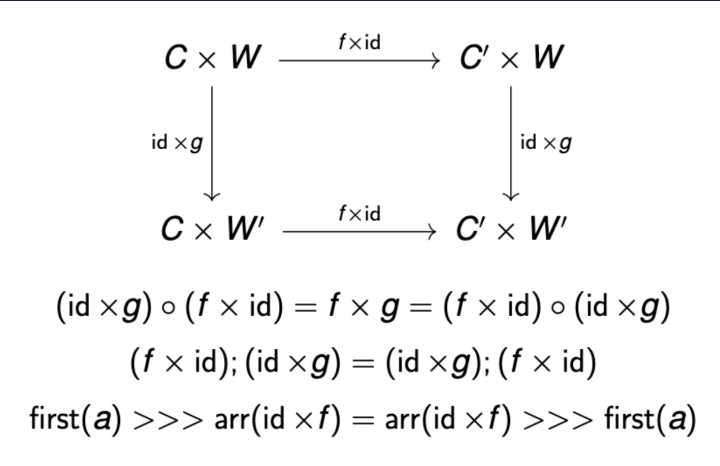
Figure 10: Arrow Laws

Two Arrow laws trivialise as a result of our example, so diagrams aren’t produced. The first such law is $\text{arr}(f;g)=\text{arr}(f)\ggg \text{arr}(g).$ For our example, this law trivialises, as $\ggg : = \text{composition}$ and $\text{arr} := \text{id}_{(Y^X)}.$ The second law to trivialise is $\text{first}(\text{arr}(f))=\text{arr}(f \times \text{id})$ since we have set $\text{first}(f) := f \times \text{id}.$

Freyd Categories

To understand Freyd categories, we must first define what a symmetric premonoidal category is.

Definition. A symmetric premonoidal category includes:

• An object $I$ (unit).
• Natural transformations that define how objects interact:
  • Associativity: $\alpha : (x \otimes y) \otimes z \to x \otimes (y \otimes z)$
  • Left unitor: $\lambda : x \otimes I \to x$
  • Right unitor: $\rho : I \otimes x \to x$
  • Symmetry: $\sigma : x \otimes y \to y \otimes x$
• All components are central .

A morphism $f : x \to x'$ is central if $\forall g:y \to y', \quad f \otimes y ; x' \otimes g = x \otimes g ; f \otimes y'$

Now, we can define a Freyd category, recalling the definition from the introduction.

Definition. A Freyd category consists of:

• A category $C$ with finite products.
• A symmetric premonoidal category $K$.
• An identity-on-objects functor $J : C \to K$ that:
  • Preserves symmetric premonoidal structure.
  • Ensures $J(f)$ is always central.

Arrows vs Freyd Categories: Similarities and Differences

At first glance, the definition of a Freyd category appears strikingly similar to that of an Arrow. This apparent similarity led to the folklore belief that they were equivalent structures.

A Freyd category consists of two categories $C$ and $K$ with an identity-on-objects functor $J: C \to K$, where: - $C$ has finite products - $K$ is symmetric premonoidal (with a functor $− \otimes z$) - $J$ maps finite products in $C$ to the premonoidal structure in $K$

In our culinary metaphor, this loosely translates to: - $C$: The idealized recipes (Haskell types and functions) - $K$: The real-world kitchen operations (computations represented by the Arrow type $\text{Ar}(x,y)$) - $J$: The translation process (via arr, embedding pure functions) - Composition in $K$: The sequencing of operations (via >>>) - Premonoidal structure in $K$: The ability to process pairs (via first)

Recalling the how we’ve interpreted Arrows in the cullinary setting, the apparent correspondence between Arrows and Fryed categories seemes quite natural. In fact, for many years the two concepts were thought to be two ways of speaking about the same thing among those in the programming languages community.

However, Atkey’s work revealed a crucial distinction: Arrows are more general than Freyd categories . The key difference lies in how they handle inputs:

• Freyd categories allow only a single input to computations
• Arrows support two separate inputs:
  • One may be structured (modeled using comonads)
  • This additional flexibility allows Arrows to represent computations that Freyd categories cannot

To bridge this gap, Atkey introduced the concept of indexed Freyd categories , which can model two structured inputs. The relationship can be summarized as: Arrows are equivalent to Closed Indexed Freyd Categories.

In our culinary metaphor, we can understand this relationship as follows: a Freyd category is like a restaurant that can only take one order at a time (a single input), while Arrows are like a more sophisticated establishment that can handle both individual orders and special requests that come with their own context (two inputs, one potentially structured). The closed indexed Freyd categories that Atkey identifies represent the perfect middle ground — restaurants that can efficiently manage multiple orders with specialized instructions while maintaining the core operational principles that make kitchens function. This is particularly valuable when preparing complex “quantum dishes” where ingredients might be entangled and interact with each other in non-local ways.

Figure 11: Arrows vs. Freyd Categories. Arrows support two inputs (one potentially structured) and are equivalent to Closed Indexed Freyd Categories, which generalize standard Freyd Categories that handle only single inputs.

This distinction helps explain why Arrows have proven particularly useful in domains like quantum computing, where managing multiple inputs with complex relationships is essential.

R. Atkey’s paper finds the relationship between Arrows and different constraints on Freyd categories as follows:

Figure 12: Relationship Between Structures

---

Key Insights: - Arrows can be defined both as monoids in categories of strong profunctors and operationally through concrete morphisms ($\text{arr}$, $\ggg$, $\text{first}$) - Freyd categories formalize the relationship between pure functions and effectful computations using symmetric premonoidal structure - Despite the folklore belief, Arrows are strictly more general than Freyd categories because they can handle two separate inputs (one potentially structured) - Arrows are equivalent to closed indexed Freyd categories, bridging the conceptual gap

---

Applications and Questions The main goal of our Adjoint School project was to structure effects in quantum programming languages using generalizations of monads. Relative monads are a popular generalization of monads. These monads need not be endofunctors, and they’re known to generalize Arrows as well. Since we already know how to structure quantum effects using Arrows, it follows that it should be theoretically possible to structure quantum effects using relative monads.

Arrows’ capacity to handle multiple inputs with a single, potentially structured output offers tractability that is particularly useful in quantum computing. Particles in quantum systems can be in entangled states, where the manipulation of one particle influences others in real time, irrespective of distance. This non-local interaction can be modeled through Arrows’ ability to combine several inputs while keeping track of their interrelationships.

Our group investigated the possibility of doing exactly this. The main technical issue arises from the fact that the way Arrows have been implemented in Haskell to structure quantum effects does not provide a categorical semantics for the problem.

For our ACT2025 presentation, we were able to construct a relative monad capable of handling classical control in the quantum setting, but the following questions still remain:

• Can one build a relative monad to model quantum effects?

• If so, how might an implementation of these ideas in Haskell compare to Arrow-based approaches?

The ride from burrito monads to Arrow kitchens has carried us farther than we anticipated, illustrating that even established mathematical folklore sometimes requires precise re-evaluation. As we continue to learn about these structures, we hope this post will motivate others to participate in the exploration of these tools and their use in quantum computing and beyond.