The n-Category Café

For example, Wikipedia defines the $L$-function of an elliptic curve $E$ this way:

$$L(E,s) = \prod_p L_p(E,s)^{-1}$$ where $$L_p(E,s) = \left\{ \begin{array}{lc} 1-a_p p^{-s}+p\cdot p^{-2s} & p \nmid N\\ 1 - a_p p^{-s} & p\mid N \; and \; p^2 \nmid N \\ 1 & p^2|N \end{array} \right.$$ where in the case of good reduction $a_p$ is $p + 1 -$ (number of points of $E$ mod $p$), and in the case of multiplicative reduction $a_p$ is ±1 depending on whether E has split (plus sign) or non-split (minus sign) multiplicative reduction at $p$. A multiplicative reduction of curve $E$ by the prime $p$ is said to be split if $-c_6$ is a square in the finite field with $p$ elements.

I won’t list all the ways this is confusing and unpleasant. The article doesn’t say what $c_6$ is! I won’t either. I’ll just say that $p$ ranges over primes and $N$ is a number called the conductor of the elliptic curve. If you follow the link and read Wikipedia’s explanation of that, you’ll enter a whole new world of pain.

Surely this can’t be the fundamental definition of the $L$-function of an elliptic curve! How could such a messy, complicated thing be fundamental? Surely this should be a theorem, where we take some simpler definition and grind out its consequences in gory detail.

I won’t actually give you what I think is a better definition of the $L$-function of an elliptic curve. Sorry! I might someday, but I still need to check that it matches this definition.

As a small step in this direction, let’s unpack the mysteries of the ‘conductor’ and transform the above definition into something easier to understand. The definition will still be extremely unpleasant. But it will involve some nice concepts about curves.

For our purposes let’s start with a lowbrow definition of an elliptic curve. Take an equation

$$y^2 = P(x)$$

where $P$ is any cubic with integer coefficients. If $P$ does not have repeated complex roots, we call this an elliptic curve. The solutions $(x,y) \in \mathbb{C}^2$ will form a smooth manifold, and in fact a smooth affine variety. If we tack on one extra point, a so-called ‘point at infinity’, we get a smooth projective variety that’s shaped like a torus.

What if $P$ has repeated roots? Then the solutions will not form a smooth variety. Two things can go wrong: we can get a cusp, or a node. For example,

$$y^2 = x^3$$

has a cusp at the origin:

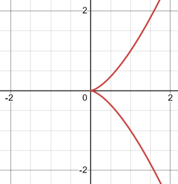
The cusp is the sharp pointy thing.

On the other hand,

$$y^2 = x^3 + x^2$$

has a node at the origin:

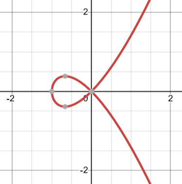
There’s a node where the curve crosses itself. Near the node the curve looks like a little X. In other words, there are two different tangent lines at a node.

So far I’ve been talking about complex solutions of

$$y^2 = P(x)$$

and drawing you real solutions. But because $P$ has integer coefficients, we can look at solutions in any field whatsoever! The $L$-function of an elliptic curve is a clever way of keeping track of how many solutions there are in every finite field. There’s one finite field $F_q$ for each prime power $q = p^n$.

The horrible definition of $L$-function given above only talks about the finite fields $F_p$, not the other finite fields involving powers of primes. That’s one reason it’s forced to be tricky and complicated. It’s trying to be ‘economical’, but premature economizing is one of the main causes of suffering in mathematics.

Okay, now let me unpack the above definition of $L$-function:

The $L$-function of an elliptic curve is defined to be $$L(E,s) = \prod_p L_p(E,s)^{-1}$$ where:

1) $L_p(E,s) = 1 - a_p p^{-s} + p^{1-2s}$ if $E$ has good reduction at $p$. This means that our elliptic curve $E$ remains smooth if we treat it as a curve over $\mathbb{F}_p$.

2) $L_p(E,s) = 1$ if $E$ has additive reduction at $p$. This means that $E$ gets a cusp if we treat $E$ as a curve over $\mathbb{F}_p$.

3) $L_p(E,s) = 1 - p^{-s}$ if $E$ has split multiplicative reduction at $p$. This means that we gets a node if we treat $E$ as a curve over $\mathbb{F}_p$, and the two tangent lines to this node have slopes that are defined in $\mathbb{F}_p$.

4) $L_p(E,s) = 1 + p^{-s}$ if $E$ has nonsplit multiplicative reduction at $p$. This means that we gets a node if we treat it as a curve over $\mathbb{F}_p$, but the two tangent lines to this node have slopes that are not defined in $\mathbb{F}_p$.

It’s still an annoying definition by cases, where each case involves an arbitrary-looking formula. Whenever a definition involves different cases, you should assume someone hasn’t precisely put their finger on the concept they’re after… or else they don’t want to tell you about it.

And of course we need purely algebraic definitions of ‘smooth’, ‘cusp’ and ‘node’ that work for algebraic curves over finite fields, for this definition to even make sense. But that’s what algebraic geometers are paid to do, so we can assume that’s been done.

More confusing to me was case 4). What the heck is a line whose slope is not defined? Here’s the deal: when you try to work out the slopes of the tangent lines to your node, you need to solve some polynomial equations. Since $\mathbb{F}_p$ is not algebraically closed, you may be unable to solve these equations in $\mathbb{F}_p$. That’s what happens in case 4). But you can always solve these equations in some algebraic extension of $\mathbb{F}_p$: that is, some bigger field $\mathbb{F}_q$ where $q = p^n$.

Next time I want to give some examples of reducing elliptic curves mod $p$. I want to illustrate some things that can happen, and how the different cases above affect patterns in the count of points not just over $\mathbb{F}_p$ but also over $\mathbb{F}_q$ where $q$ is any power of $p$.

I also want to say what this ‘additive’ and ‘multiplicative’ jargon is all about!