The n-Category Café

To recap, we saw that the process of taking the index defines an order-embedding

$$Index: \text{(infinite sets)} \hookrightarrow \text{(well-ordered sets)}.$$

So

$$X \lt Y \implies Index(X) \prec Index(Y),$$

and therefore

$$Index(X) \cong Index(Y) \implies X \cong Y.$$

So if a well-ordered set $W$ is isomorphic to $Index(X)$ for some infinite set $X$, then $X$ is determined uniquely up to isomorphism, and we write $X = \aleph_W$. In that case, I’ll say $\aleph_W$ exists.

For natural numbers $n$, there’s exactly one well-ordered set with $n$ elements; call it $\mathbf{n}$. We write $\aleph_{\mathbf{n}}$ as $\aleph_n$. For example:

• $\aleph_0$ is the unique infinite set whose index is the empty well-ordered set $\mathbf{0}$; that is, $\aleph_0 \cong \mathbb{N}$.

• $\aleph_1$ is the unique infinite set whose index is the one-element well-ordered set $\mathbf{1}$. That is, up to isomorphism, there is exactly one infinite set smaller than $\aleph_1$. So $\aleph_1$ is $\mathbb{N}^+$, the smallest set $\gt \mathbb{N}$.

The assignments $Index$ and $\aleph_\bullet$ are mutually inverse:

$$\aleph_{Index(X)} \cong X$$

for infinite sets $X$, and

$$Index(\aleph_W) \cong W$$

for well-ordered sets $W$ such that $\aleph_W$ exists. Set theory books sometimes contain the statement “every infinite set is an aleph”; the first of these isomorphisms is our version of this.

For want of a better word, let’s say that a well-ordered set $W$ is alephable if $\aleph_W$ exists. Then the inverse processes $Index$ and $\aleph_\bullet$ define an equivalence

$$(\mathbf{Set}_\infty, \leq) \simeq (\text{alephable well-ordered sets}, \preceq).$$

ZFC-based set theory puts the emphasis on the right-to-left assignment, $W \mapsto \aleph_W$. In ZFC, every well-ordered set is alephable, so that’s a reasonable thing to do. But in ETCS, where that’s not guaranteed, it makes more sense to emphasize the left-to-right direction, $X \mapsto Index(X)$. That’s why I started there.

I chose the word “index” as an abbreviation for “aleph-index”: the index of $X$ is the well-ordered set $W$ such that $\aleph_W \cong X$. Maybe set theorists have no name for “index” because they’d just say “the ordinal $\alpha$ such that $X = \aleph_\alpha$”.

Incidentally, the reason why I switched from $K(X)$ to $Index(X)$ near the start of the last post was exactly so that we’d get an inverse to $\aleph_\bullet$. I’d have been happy to stick with $K(X)$ (thus, also including the finite sets $\lt X$) if there was a standard name for the inverse to $K$. That inverse would be a ladder of sets like the alephs, but starting at $\emptyset$ rather than $\mathbb{N}$. But as far as I know, it doesn’t have a name (and in particular, it’s not quite the same as the von Neumann hierarchy).

Which well-ordered sets $W$ are alephable? This is the same as the question “which well-ordered sets are the index of some set?”, which we already answered last time. Translating into the language of alephs, we know:

• $0$ is alephable (i.e. $\aleph_0 \cong \mathbb{N}$ exists);

• if $W$ is alephable then so is $W^+$, and $\aleph_{W^+} \cong (\aleph_W)^+$;

• if $W$ is alephable then so is $V$ for all $V \prec W$.

The first two properties guarantee that $\aleph_n$ exists for all natural numbers $n$. But $\aleph_W$ need not exist for all well-ordered sets $W$. In particular:

It is consistent with ETCS that $\aleph_\omega$ does not exist.

This is just a restatement of a fact we met last time: it is consistent with ETCS that there is no set with index $\omega$. What it tells us that if there are any models of ETCS at all, there is one in which the only sets are

$$0, 1, 2, \ldots, \aleph_0, \aleph_1, \aleph_2, \ldots.$$

That’s it. No more!

There’s a crucial characterization of the alephs that doesn’t mention index:

If $\aleph_W$ exists, then so does $\aleph_V$ for every $V \prec W$, and $\aleph_W$ is the smallest set $\gt \aleph_V$ for every $V \prec W$.

For example, if $\aleph_\omega$ exists then it is the smallest set with the property that $\aleph_\omega \gt \aleph_n$ for every $n \in \mathbb{N}$.

To see why this characterization holds, think about the order-equivalence

$$(\mathbf{Set}_\infty, \leq) \simeq (\text{alephable well-ordered sets}, \preceq).$$

We know that among all well-ordered sets, the alephable ones are downwards closed. Now, it’s a triviality that any well-ordered set $W$ is the least well-ordered set $\succ V$ for every $V \prec W$. Transporting this trivial fact across the equivalence, from right to left, gives the characterization of $\aleph_W$.

When people choose to denote a set by $\aleph_W$ rather than just $X$ or whatever, it’s usually because they want to see it as part of the succession of alephs

$$\aleph_0, \aleph_1, \ldots, \aleph_\omega, \aleph_{\omega + 1}, \ldots.$$

The beginning part of that succession of alephs is displayed in what I called the “tautological bundle”. Last time I drew this picture for a set $X$, where the fibre over an isomorphism class $[A]$ is $A$ itself:

If instead we start with an alephable well-ordered set $W$ and put $X = \aleph_W$, the picture becomes this:

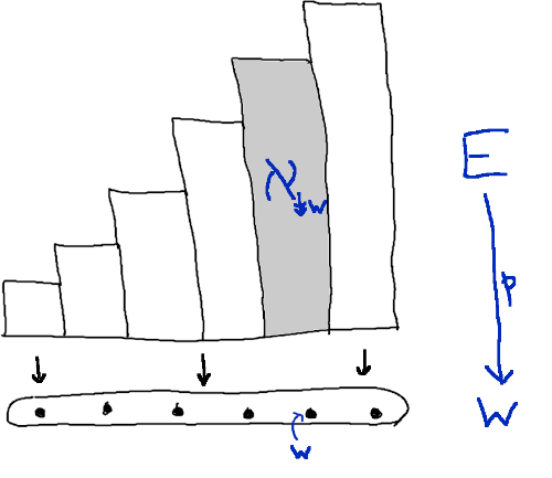
Here I’ve used the notation

$$↡ w = \{ v \in W : v \lt w \}$$

when $w \in W$. It’s standard to write $\downarrow w$ for the set of elements less than or equal to $w$; this is a variation on that notation. (If you want to use the double downwards arrow in the comments, I’m afraid the only way I know of getting it here is to use unicode: type “↡” without the quotation marks.)

Every downwards closed proper subset of $W$ is of the form $↡ w$ for a unique $w \in W$. Equivalently, every well-ordered set $\prec W$ is isomorphic to $↡ w$ for a unique $w \in W$. So the fibres of $p: E \to W$ are the alephs $\aleph_V$ for $V \prec W$.

The alephs that appear as the fibres here stop one short of $\aleph_W$ itself. If we want to get $\aleph_W$ as a fibre, we can do it by replacing $W$ by $W^+$. Then the picture is:

Here I’ve lazily reused the letters $E$ and $p$, which I shouldn’t really have done: they’re different from the $E$ and $p$ for $W$. Anyway, the point is that the top fibre here is $\aleph_W$.

All this gives another characterization of the alephs. Let $W$ be a well-ordered set. Then $\aleph_W$ exists if and only if there exist a set $E$ and function $p: E \to W^+$ with the following property:

for all $w \in W^+$, the fibre $p^{-1}(w)$ is the smallest infinite set $\gt p^{-1}(v)$ for all $v \lt w$.

In that case, $p: E \to W^+$ is determined uniquely up to isomorphism of sets over $W^+$, and the fibre over the top element of $W^+$ is $\aleph_W$.

Summarizing what we’ve just seen and what we saw at the end of the last post, the following conditions on a model of ETCS are equivalent:

• all alephs exist;

• every well-ordered set is the index of some set;

• the “Cantorian axiom”: for every well-ordered set $W$, there exists a function $p: E \to W$ into $W$ such that for all $w \in W$, the fibre $p^{-1}(w)$ is the smallest infinite set $\gt p^{-1}(v)$ for all $v \lt w$;

• for every set $I$, there exists a function into $I$ whose fibres are pairwise non-isomorphic.

I’ll finish by relating the condition “all alephs exist” to the existence of limits (which we met in Part 2). First:

All alephs exist implies unboundedly many weak limits.

“Unboundedly many” means that for every set $X$, there is some weak limit at least as big as $X$.

Why is this true, assuming all alephs exist?

Let $X$ be an infinite set. We can take an initial well-ordered set $W$ with underlying set $X$. I claim that $\aleph_W$ does the job: that it’s a weak limit $\geq X$.

First, $\aleph_W$ is a weak limit. “Initial” means that $W$ is the least well-ordered set of its cardinality, so $W$ can’t be a successor. Hence $W$ is a limit (as a well-ordered set). Now we saw last time that a set is a weak limit if and only if its index is a limit. Put another way, $\aleph_V$ is a weak limit if and only if $V$ is a limit, for well-ordered sets $V$. So $\aleph_W$ is a weak limit.

All we have left to do is to show that $\aleph_W \geq X$. By construction, the underlying set $U(W)$ of $W$ is $X$, so our task is to show that

$$\aleph_W \geq U(W).$$

This looks like this should be true by miles: after all, $\aleph_0 = \mathbb{N}$ is much bigger than $\emptyset$, and $\aleph_1$ is vastly bigger than $1$, and $\aleph_\omega$ is dramatically bigger than $U(\omega) = \mathbb{N}$, etc. In a couple of posts’ time, we’ll look in detail at the question of $\aleph_W$ versus $U(W)$. In any case, the inequality we have to prove follows from the inequality $K \preceq I$ mentioned near the start of the last post. I’m running out of steam now so I won’t explain how, but it only takes a couple of lines.

So, if all alephs exist then there are unboundedly many weak limits. What about the converse? It’s false:

It is consistent with ETCS + (there are unboundedly many weak limits) that not all alephs exist.

In other words, “all alephs exist” is strictly stronger than “there are unboundedly many weak limits”.

For the proof, I’ll want to talk not only about weak limits and alephs, but also strong limits and beths. So that’s going to have to wait until next time.

Next time

There are two standard ways to make a set $X$ bigger: take its successor $X^+$ or its power set $2^X$. The alephs are what you get by starting with $\mathbb{N}$ and repeatedly taking successors. The beths are what you get by starting with $\mathbb{N}$ and repeatedly taking power sets. We’ll meet the beths next time.