The n-Category Café

The definition

Let’s have a quick look at the definition first: this is a typical piece of homological algebra. For each graph $G$ we define a $k$-chain on $G$ to be a $k+1$-tuple of vertices of $G$ such that adjacent vertices are distinct: $$(a_{0},\dots ,a_{k}),\quad a_{i}\in \mathrm{Vertices}(G),\quad a_{i}\ne a_{i+1}.$$ We equip the graph with the path length metric, so each edge has length $1$, and we define the length of a chain to be the length of the path obtained by traversing its vertices: $$\ell ((a_{0},\dots ,a_{k}))\coloneqq \sum _{i=0}^{k-1}d(a_{i},a_{i+1}).$$ The chain group $\mathrm{MC}_{k,l}(G)$ is defined to be the free abelian group on the set of $k$-chains of length $l$. We define the differential $\partial \colon \mathrm{MC}_{k,l}\to \mathrm{MC}_{k-1,l}$ by $\partial \coloneqq \sum (-1)^{i}\partial _{i}$ where $$\partial _{i}(a_{0},\ldots ,a_{k}) \coloneqq \begin{cases} (a_{0},\ldots ,\widehat{a_{i}},\ldots ,a_{k}) & \mathrm{if } \ell (a_{0},\ldots ,\widehat{a_{i}},\ldots ,a_{k})=l, \\ 0 & \mathrm{otherwise}. \end{cases}$$ Here, as usual, $\widehat{x}$ means “omit $x$”. The graph magnitude is then defined to be the homology of this differential: $$\mathrm{MH}_{k,l}(G)\coloneqq \mathrm{H}_{k}(\mathrm{MC}_{\ast ,l}(G),\partial ).$$ Unfortunately, I don’t know of any intuitive interpretation of the chain groups.

Functoriality

One standard advantage of this sort of categorification is that it has functoriality where the original invariant did not. We don’t usually have morphisms between numbers or polynomials, but we do have morphisms between groups. In the case here we have the category of graphs with the morphisms sending vertices to vertices with edges either preserved or contracted, and graph magnitude homology gives a functor from that to the category of bigraded groups and homomorphisms.

Categorifying properties of magnitude

Here are some of the properties of magnitude that we can categorify. With the exception of disjoint unions, all of the other categorification results require some decidedly non-trivial homological algebra to prove.

Disjoint unions

Tom showed that magnitude is additive with respect to the disjoint union of graphs: $$#(G\sqcup H) = #G + #H.$$ Our categorification of this is the additivity of the magnitude homology: $$\mathrm{MH}_{\ast ,\ast }(G\sqcup H) \cong \mathrm{MH}_{\ast ,\ast }(G) \oplus \mathrm{MH}_{\ast ,\ast }(H).$$

Products

Tom showed that magnitude is multiplicative with respect to the cartesian product $\square$ of graphs $$#(G\Box H) = #G\cdot #H.$$ The categorification of this is a Künneth Theorem which says that there is a non-naturally split, short exact sequence: $$\begin{aligned} 0\to \mathrm{MH}_{\ast ,\ast }(G)\otimes \mathrm{MH}_{\ast ,\ast }(H) \to \mathrm{MH}_{\ast ,\ast }(G\square H)\\ \to \mathrm{Tor}\bigl (\mathrm{MH}_{\ast +1,\ast }(G), \mathrm{MH}_{\ast ,\ast }(H)\bigr ) \to 0. \end{aligned}$$ If either $G$ or $H$ has torsion-free magnitude homology, then this sequence reduces to an isomorphism $$\mathrm{MH}_{\ast ,\ast }(G{\square }H)\cong \mathrm{MH}_{\ast ,\ast }(G)\otimes \mathrm{MH}_{\ast ,\ast }(H).$$ Despite quite a bit of computation, we don’t know whether any graphs have torsion in their magnitude homology.

Unions

Tom showed that a form of the inclusion-exclusion formula holds for certain graphs. We need a pile of definitions first.

Definition. A subgraph $U\subset X$ is called convex if $d_{U}(u,v)=d_{X}(u,v)$ for all $u,v\in U$.

One way of reading this is that for $u$ and $v$ in $U$ there is a geodesic joining them that lies in $U$.

Definition. Let $U\subset X$ be a convex subgraph. We say that $X$ projects to $U$ if for every $x\in X$ that can be connected by an edge-path to some vertex of $U$, there is $\pi (x)\in U$ such that for all $u\in U$ we have $$d(x,u) = d(x,\pi (x)) + d(\pi (x),u).$$

For instance, a four-cycle graph projects to any edge, whereas a five cycle does not project to an edge.

Definition. A projecting decomposition is a triple $(X;G,H)$ consisting of a graph $X$ and subgraphs $G$ and $H$ such that

• $X=G\cup H$,

• $G\cap H$ is convex in $X$,

• $H$ projects to $G\cap H$.

Tom showed that if $(X;G,H)$ is a projecting decomposition then $$#X +# (G\cap H)= #G +#H .$$ Our categorification of this result is that if $(X;G,H)$ is a projecting decomposition, then there is a naturally split short exact sequence $$0\to \mathrm{MH}_{\ast ,\ast }(G\cap H)\to \mathrm{MH}_{\ast ,\ast }(G)\oplus \mathrm{MH}_{\ast ,\ast }(H)\to \mathrm{MH}_{\ast ,\ast }(X)\to 0$$ (which is a form of Mayer-Vietoris sequence) and consequently there is a natural isomorphism $$\mathrm{MH}_{\ast ,\ast }(X)\oplus \mathrm{MH}_{\ast ,\ast }(G\cap H) \cong \mathrm{MH}_{\ast ,\ast }(G)\oplus \mathrm{MH}_{\ast ,\ast }(H).$$

Diagonality

Tom noted many examples of graphs which had magnitude with coefficients which alternate in sign; these examples included complete graphs, complete bipartite graphs, forests and graphs with up to four vertices.

Our categorification of this is that in all of these cases the magnitude homology is supported on the diagonal: we say a graph $G$ is diagonal if $\mathrm{MH}_{k,l}(G)=0$ if $k\neq l$. In this case the magnitude is given by $$#G=\sum _{l\geq 0}(-1)^{l}\cdot \mathrm{rank}\mathrm{MH}_{l,l}(G)\cdot q^{l},$$ and it means in particular that the coefficients of the magnitude alternate in sign.

The join $G\star H$ of graphs $G$ and $H$ is obtained by adding an edge between every vertex of $G$ and every vertex of $H$. This is a very drastic operation, for instance the diameter of the resulting join is at most $2$.

Theorem. If $G$ and $H$ are non-empty graphs then the join $G\star H$ is diagonal.

This tells us immediately that complete graphs and complete bipartite graphs are diagonal. Together with the other properties of magnitude homology mentioned above, we recover the alternating magnitude property of all the graphs noted by Leinster, as well as many more.

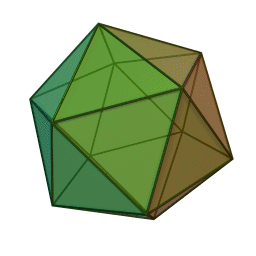
However, there is one graph that appears to be diagonal, at least up to degree $7$ according to our computer calculations but which we can’t prove is diagonal, i.e. it doesn’t follow from the results above. This graph is the icosahedron graph which is the one-skeleton of the icosahedron.

Where next?

There are plenty of questions that you can ask about magnitude homology, a fundamental one is whether there are graphs with the same magnitude but different magnitude homology and a related one is whether you can categorify Tom’s result (conjectured by me and David Speyer) on the magnitude of graphs which differ by certain Whitney twists.

One interesting thing demonstrated here is that magnitude has its tendrils in homological algebra, yet another area of mathematics to add to the list which includes biodiversity, enriched category theory, curvature and Minkowski dimension.