The n-Category Café

Today, all vector spaces are over $\mathbb{C}$ and finite-dimensional. Most (all?) of what I’ll say can be done in more sophisticated functional-analytic settings, but I’ll stick to this most basic of situations.

Fix a vector space $X$ equipped with an inner product. By an operator on $X$, I mean a linear map $X \to X$.

Here’s how the analogy goes.

Complex numbers are like operators  This is the basis of everything that follows.

There’s not much substance to this statement yet. For now, let’s just observe that both the complex numbers and the operators on $X$ form rings. I’ll write $End(X)$ for the ring of operators on $X$, following the usual categorical custom. (“End” stands for “endomorphisms”.)

The two rings $\mathbb{C}$ and $End(X)$ don’t seem very similar. Unlike $\mathbb{C}$, the ring $End(X)$ isn’t commutative and usually has nontrivial zero-divisors. (Indeed, as long as $dim(X) \geq 2$, there is some $T \in End(X)$ with $T \neq 0$ but $T^2 = 0$.) Perhaps surprisingly, these differences don’t prevent the development of this useful analogy.

In some loose sense, we can pass back and forth between $\mathbb{C}$ and $End(X)$. In one direction, starting with a complex number $\lambda$, we get the operator $x \mapsto \lambda x$. In elementary texts, this operator is often written as $\lambda I$, but I’ll almost always write it as just $\lambda$.

In the opposite direction, starting with an operator on $X$, we get not just a single complex number but a collection of them — namely, its eigenvalues.

Complex conjugates are like adjoints  Every complex number $z$ has a complex conjugate $z^\ast$. Taking complex conjugates defines a self-inverse automorphism of the ring $\mathbb{C}$.

Every linear map $T: X \to Y$ of inner product spaces has an adjoint $T^\ast: Y \to X$, characterized by the equation $\langle T x, y \rangle = \langle x, T^\ast y \rangle$. In particular, every operator $T$ on $X$ has an adjoint $T^\ast$, also an operator on $X$.

It’s almost true that taking adjoints defines a self-inverse automorphism of $End(X)$. The only obstruction is that taking adjoints reverses the order of composition: $(T S)^\ast = S^\ast T^\ast$. So actually, taking adjoints defines a pair of mutually inverse ring isomorphisms

$$End(X)^{op} \stackrel{\longrightarrow}{\leftarrow} End(X)$$

where $End(X)^{op}$ is the ring $End(X)$ with its order of multiplication reversed.

What about those back-and-forth passages between complex numbers and operators?

First, start with a complex number $\lambda$; then the adjoint of the operator $\lambda I$ is $\lambda^\ast I$. That is, $(\lambda I)^\ast = \lambda^\ast I$. This is why I’m writing $z^\ast$ for the complex conjugate of $z$, rather than the more common $\bar{z}$.

Second, start with an operator $T$. Then the eigenvalues of $T^\ast$ are exactly the conjugates of the eigenvalues of $T$. Why? Because taking the adjoint defines an isomorphism of rings, so $T - \lambda$ is invertible iff $(T - \lambda)^\ast = T^\ast - \lambda^\ast$ is.

Real numbers are like self-adjoint operators  A complex number $z$ is real if and only if $z = z^\ast$. By definition, an operator $T$ is self-adjoint if and only if $T = T^\ast$.

Again, let’s look at the passages back and forth between $\mathbb{C}$ and $End(X)$. First, let $\lambda \in \mathbb{C}$. As long as $X$ is nontrivial, the operator $\lambda$ is self-adjoint iff $\lambda$ is real.

Second, if $T$ is a self-adjoint operator then all its eigenvalues are real. The converse isn’t true: an operator can have all real eigenvalues without being self-adjoint. We’ll come back to that.

Any even half-serious endeavour involving self-adjoint operators makes use of the theorem that classifies them, the spectral theorem. Loosely put, this states that every self-adjoint operator is an orthogonal sum of self-adjoint operators of the most simple kind: scalar multiplication by a real number.

Precisely: given any self-adjoint operator $T$, there is a unique orthogonal decomposition $X = \bigoplus_{\lambda \in \mathbb{R}} X_\lambda$ such that for each $\lambda$, the restriction of $T$ to $X_\lambda$ is multiplication by $\lambda$. Of course, all but finitely many of these subspaces $X_\lambda$ are trivial, the nontrivial ones are those for which $\lambda$ is an eigenvalue, and $X_\lambda$ is the eigenspace $ker(T - \lambda)$.

Nonnegative real numbers are like positive operators  For a complex number $z$, the following are equivalent:

• (1) $z$ is nonnegative, i.e. real and $\geq 0$
• (2) $z = w^\ast w$ for some complex $w$
• (3) $z = w^\ast w$ ($= w^2$) for some real $w$
• (4) $z = w^\ast w$ ($= w^2$) for some nonnegative $w$
• (5) $z = w^\ast w$ ($= w^2$) for a unique nonnegative $w$.

I’ll follow custom and say that an operator $T$ is positive if it is self-adjoint and each eigenvalue is $\geq 0$. (Other names are “positive semidefinite” and “nonnegative definite”. As we were recently discussing, the terminology around positive/nonnegative is a bit of a mess.) Note that by definition, “positive” includes “self-adjoint”. This is just like the convention that when we call a complex number “nonnegative”, we tacitly include the condition “real”.

For an operator $T$ on $X$, the following are equivalent:

• (1) $T$ is positive, i.e. self-adjoint and each eigenvalue is $\geq 0$
• (1.5) $T$ is self-adjoint and $\langle T x, x \rangle \geq 0$ for all $x \in X$
• (2) $T = S^\ast S$ for some inner product space $Y$ and linear map $S: X \to Y$
• (2.5) $T = S^\ast S$ for some operator $S$ on $X$
• (3) $T = S^\ast S$ ($= S^2$) for some self-adjoint operator $S$
• (4) $T = S^\ast S$ ($= S^2$) for some positive operator $S$
• (5) $T = S^\ast S$ ($= S^2$) for a unique positive operator $S$.

The implications $5 \Rightarrow 4 \Rightarrow \cdots \Rightarrow 1$ are all either trivial or easy. The remaining implication, $1 \Rightarrow 5$, follows from the spectral theorem, using $1 \Rightarrow 5$ of the result on nonnegativity of numbers.

In particular, given $\lambda \in \mathbb{C}$, the operator $\lambda$ is positive iff the number $\lambda$ is nonnegative (assuming that $X$ is nontrivial). And given an operator $T$, if $T$ is positive then each eigenvalue of $T$ is nonnegative (but not conversely).

The modulus of a complex number is like… the modulus of an operator? What is the modulus of a complex number? Let’s answer this carefully, using the theorem above on nonnegativity of complex numbers. Let $z \in \mathbb{C}$. By the theorem, $z^\ast z$ is nonnegative, so by the theorem again, there is a unique nonnegative $m$ such that $z^\ast z = m^\ast m$ ($= m^2$). This $m$ is, of course, $\left|z\right|$, the modulus of $z$.

What is the analogue for operators? Let’s use the theorem above on positivity of operators. Let $T \in End(X)$. By the theorem, $T^\ast T$ is positive, so by the theorem again, there is a unique positive $M$ such that $T^\ast T = M^\ast M$ ($= M^2$). I’ll call $M$ the modulus of $T$ and write it as $\left|T\right|$. I don’t know whether the term “modulus” is standard here, and I’m pretty sure the notation $\left|T\right|$ isn’t — it’s risky, given the potential for confusion with a norm. But I’ll use it anyway, to emphasize the analogy.

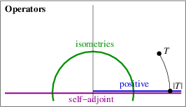
Complex numbers of unit modulus are like isometries  A complex number $z$ has unit modulus if and only if $z^\ast z = 1$, if and only if $z z^\ast = 1$. An operator $T$ is an isometry if and only if $T^\ast T = 1$, if and only if $T T^\ast = 1$ (if and only if $T$ preserves inner products, if and only if $T$ preserves distances). Isometries are more often called unitary operators, but I find the term “isometry” more vivid.

Now that we have a definition of “modulus” for operators, we can ask: which operators are literally “of unit modulus”? In other words, which operators $T$ satisfy $\left|T\right| = 1$? Here $1$ is the identity operator. Certainly $1$ is positive, so $\left|T\right| = 1$ if and only if $T^\ast T = 1^\ast 1$, if and only if $T$ is an isometry. So the different parts of the analogy hang together nicely.

Once again, let’s go back and forth between complex numbers and operators. Given $\lambda \in \mathbb{C}$, the operator $\lambda$ is an isometry iff the number $\lambda$ is of unit modulus (again, assuming that $X$ is nontrivial). Given an operator $T$, if $T$ is an isometry then all its eigenvalues are of unit modulus. Again, the converse is false, and again, we’ll come back to that.

Polar decomposition of complex numbers and operators Any complex number $z$ can be expressed as a product

$$z = u p$$

where $u$ is of unit modulus and $p$ is nonnegative. Moreover, this $p$ is uniquely determined as $\left|z\right|$, and if $z \neq 0$ then $u$ is uniquely determined by $z$ too. (If $z = 0$ then many choices of $u$ are possible.)

Similarly, it’s a theorem that any operator $T$ can be expressed as a composite

$$T = U P$$

where $U$ is an isometry and $P$ is positive. Moreover, this $P$ is uniquely determined as $\left| T \right|$, and if $T$ is invertible then $U$ is uniquely determined by $T$ too. (If $T$ is not invertible then many choices of $U$ are possible.)

In the case where $T$ is just multiplication by a scalar $z$, the second theorem (polar decomposition of operators) reduces to the first (polar decomposition of complex numbers).

If you prefer, you can decompose an operator in the other order too: an isometry followed by a positive operator. To see this, decompose $T^\ast$ as $U P$; then $T = P^\ast U^\ast = P U^\ast$. But $U^\ast$ is an isometry, since the adjoint of an isometry is again an isometry — just as the conjugate of a complex number of unit modulus is again of unit modulus.

And that’s the analogy.

Normal operators, and the fraying of the analogy

Like all analogies, this one eventually frays. Right at the start, we noted a big difference between complex numbers and operators: multiplying complex numbers is commutative, but composing operators isn’t. And another one: there are no nonzero nilpotent complex numbers, but there are nonzero nilpotent operators.

I’ll explain the trouble this causes by talking about operators $T$ that satisfy the equation $T^\ast T = T T^\ast$. In a fit of no inspiration, someone once called such operators normal, and the name stuck.

Now, all complex numbers $z$ are “normal”, in the sense that $z^\ast z = z z^\ast$, but not all operators $T$ are normal — for example, any nonzero nilpotent is “abnormal”. So this is a wrinkle in the analogy. You might conclude from this that the correct analogue for the complex numbers is not the set of all operators, but just the normal ones. This idea has in its favour that all self-adjoint operators and isometries (“real numbers” and “numbers of unit modulus”) are normal — because an operator commutes with both itself and its inverse.

However, the normal operators don’t form a ring, at least, not under the usual operations. The class of normal operators is closed under taking polynomials in one variable, but not under composition. Indeed, the polar decomposition theorem implies that by composing two normal operators, we can obtain any operator we like.

The normal operators are nevertheless a useful class, giving further depth to the analogy. I clearly remember the first time I saw the definition of normal operator: I was overwhelmed by the feeling that it was an awful hack. “Someone,” I thought to myself, “simply wants a definition that includes both self-adjoint operators and isometries, and they’ve written down the first thing that came into their head.” Oh young, foolish self; I was wrong. Here’s why:

Normal operators are exactly the right context for the spectral theorem.

Recall that for an operator $T$, the spectral theorem says that $X$ is the orthogonal sum of the eigenspaces of $T$. This statement isn’t true for all operators. Earlier on, I stated that it was true for all self-adjoint operators, and that in that case, all the eigenvalues are real. But there are certainly non-self-adjoint operators such that $X$ is the orthogonal sum of the eigenspaces — multiplication by any non-real scalar is an example.

So which operators is the spectral theorem true for? Exactly the normal ones. In other words:

Spectral theorem  Let $T$ be an operator on $X$. Then $X$ is the orthogonal sum of the eigenspaces of $T$ if and only if $T$ is normal.

This says that multiplication by a scalar is a normal operator, that the class of normal operators is closed under orthogonal sums, and that combining these two constructions generates all possible normal operators. ‘Only if’ is easy; it’s ‘if’ that takes work. You can find a proof in Linear Algebra Done Right.

We can read off two corollaries, both supporting the claim that “complex numbers are like normal operators” is a better analogy than “complex numbers are like operators”.

Corollary  Let $T$ be a normal operator. Then (i) $T$ is self-adjoint if and only if all eigenvalues of $T$ are real, and (ii) $T$ is an isometry if and only if all eigenvalues of $T$ are of unit modulus.

We saw earlier that without the normality, the “only if” parts are true but the “if” parts fail.

Fundamental theorem of algebra for normal operators  Let $p$ be a nonconstant polynomial over $\mathbb{C}$, and let $T$ be a normal operator. Then there exists a normal operator $S$ such that $p(S) = T$.

For both proofs, all we have to do is observe that the class of operators $T$ for which the result holds contains all operators of the form “multiply by a scalar” and is closed under orthogonal sums. That’s all there is to it!