The n-Category Café

The following five snapshots of the spread are more-or-less independent of each other.

Diversity

The definition of spread was motivated by Tom Leinster and Christina Cobbold’s definition of diversity measures for ecosystems in which they take into account the relative abundances of the species and the relatedness of each pair of species, or in math-speak, we can use these to assign a number to each finite metric space with a probability measure on it – the points represent the species, the metric describes the relatedness and the probability measure describes the relative abundances.

Tom and Christina give us a diversity measure for each number $q$ with $0\le q \le\infty$, so for a finite metric space we can use the uniform probabiltiy measure on it and take the diversity measure for $q=0$: that is precisely the spread.

The more classical version of the Tom and Christina’s measures – the Hill numbers – only takes into account relative abundances of species and not the relatedness of species, so these are defined for probability spaces with no metric on them (or with the discrete metric on them, if you prefer). In that case, the $q=0$ diversity measure is just the number of species present. So from that point of view, the spread can be seen as an analogue of the number of species in an ecosystem.

Basic behaviour

If $X$ is a finite metric space with $N$ points, $t \gt 0$ and $t X$ denotes $X$ with the metric scaled by a factor of $t$ then we get the following basic properties of the spread.

• $1\le E_0(X)\le N$;
• $E_0(t X)$ is increasing in $t$;
• $E_0(t X)\to 1$ as $t\to 0$;
• $E_0(t X)\to N$ as $t\to \infty$;
• $E_0(X)\le e^{diam(X)}$.

For instance, if $t R$ is the following three-point metric space

then we get the following plot of the spread as we scale $t$.

So when the space is scaled very small it looks like there is one point, at medium scales it looks like there are two points, and at large scales all three points are distinctly visible.

Magnitude

Long-time readers of this blog will not be surprised to hear that spread is connected to Tom Leinster’s notion of magnitude (called cardinality in some early blog posts). The magnitude $|X|$ of a metric space $X$ is not always defined; for instance, Tom showed that there is no magnitude defined for a certain scaling of the five-point metric space coming from the complete bipartite graph $K_{3,2}$. If we plot the magnitude of the scalings of this space together with the spread of these scalings then we see that the spread is rather more nicely behaved!

Tom Leinster said he thinks this shows that the spread is more suave than the magnitude.

For well-behaved metric spaces the magnitude is an upper bound for the spread – in this case ‘well behaved’ means ‘positive definite’ and such spaces include subspaces of Euclidean space. For homogeneous metric spaces the magnitude and the spread actually coincide.

Dimension

As we have a notion of size, we can associate a notion of dimension.

• If we scale a line by a factor of $t$ then its length (its size) scales by a factor of $t^1$.

• If we scale a rectangle by a factor of $t$ then its area (its size) scales by a factor of $t^2$.

• If we scale a cuboid by a factor of $t$ then its volume (its size) scales by a factor of $t^3$.

Of course, the $1$, $2$ and $3$ appearing there are our usual concept of dimension of those three spaces. So given a notion of size of metric spaces, the associated dimension of a metric space is the growth rate of the size. One has to be precise about what growth rate is here, but you can think of it as the (instantaneous) slope of the log-log plot of size versus scale.

In particular, the spread dimension $dim_0(X)$ of a metric space $X$ is defined by

$$dim_0(X)\,\coloneqq\, \left.\frac{\mathrm{d} \,log(E_0(t X))}{\mathrm{d} \,log(t)}\right|_{t=1} \, =\, \left.\frac{t}{E_0(t X)}\frac{\mathrm{d}E_0(tX)}{\mathrm{d}t}\right|_{t=1}.$$

This notion of spread dimension is scale dependent, but that is not unreasonable. Think of a very long and very thin rectangle. If it is scaled very, very small you might think it looks like a point, so is zero-dimensional. As it is scaled up you start to notice its length but not its width, so it seems one-dimensional. As it is scaled even more it finally looks two-dimensional. If this rectangle is actually made from, say, atoms, then if it scaled even more then you start to see the individual points and it begins to look zero-dimensional again.

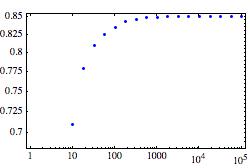
We can numerically calculate the spread dimension for a rectangle of $10$ by $4900$ points at various scales, and the above describes exactly the kind of phenomena that we see.

If my computer could handle much bigger matrices then I could calculate the dimension profile for say $1000$ by $100000000$ points and see a much more pronounced step-like behaviour from zero to one to two to zero dimensions.

We don’t have to stick to boring old shapes like rectangles. We can try fractals! We can take a finite metric space with lots of points which approximates say the Koch curve, get maple to calculate the spread dimension at various scales and plot the result. At medium scales the spread dimension is shockingly close to the Hausdorff dimension of the Koch curve, namely $ln 4/ ln 3$. So when it’s not too small and it’s not too large, then the finite approximation looks ‘Koch-like’.

The same phenomemon is seem for finite approximations to Cantor sets and Sierpinski triangles, so there seems to be some geometric content to the spread dimension.

Non-finite metric spaces

There is an obvious way to generalize the notion of spread to a non-finite metric space $X$ provided that the metric space comes equipped with a canonical measure $\mu$ such that the total measure of the space is finite. In that case we just define the spread as follows.

$$E_0(X)\coloneqq\int_{x\in X} \frac{\mathrm{d}\mu(x)}{\int_{y\in X} e^{-d(x,y)} \,\mathrm{d}\mu(y)}.$$

From that one can calculate the spread of a length $\ell$ straight line segment and of an $n$-sphere with radius $R$. As it’s getting late, I won’t put the details here, but let the interested reader find out the answers by looking in the paper.

One class of metric spaces with a canonical measure is the class compact Riemannian manifolds. For this class of spaces it is possible to calculate the leading order terms in the asymptotic behaviour of the spread as a space $M$ is scaled up. These leading order terms depends just on the volume $vol(M)$ and the total scalar curvature $tsc(M)$, in particular we have the following.

$$E_0(t M) = \frac{1}{n!\,\omega_n}\left(t^n vol(M) + \frac{n+1}{6}t^{n-2} tsc(M) +O(t^{n-4})\right) \quad \text{as }\quad t\to\infty,$$

where $\omega_n$ is the volume of the unit $n$-ball.

In particular, for a Riemannian surface $\Sigma$ we have:

$$E_0(t\Sigma)=\frac{area(\Sigma)}{2\pi}t^2+\chi(\Sigma)+O(t^{-2})\quad \text{as } \quad t\to\infty,$$

where $\chi$ is the Euler characteristic.

Final comments

In conclusion, it seems that this easy to write down measure of size of a metric space has many interesting properties.