This Week’s Finds in Mathematical Physics (Week 292)
Posted by John Baez
.")
In week292 of This Week’s Finds, learn about Henry Paynter’s “bond graphs” — diagrams that engineers use to model systems made of mechanical, electronic, and/or hydraulic components: springs, gears, levers, pulleys, pumps, pipes, motors, resistors, capacitors, inductors, transformers, amplifiers, and so on. And learn how different classes of systems like this call for different kinds of mathematics: symplectic geometry, complex analysis, and even a bit of Hodge theory.
Posted at January 30, 2010 5:12 AM UTC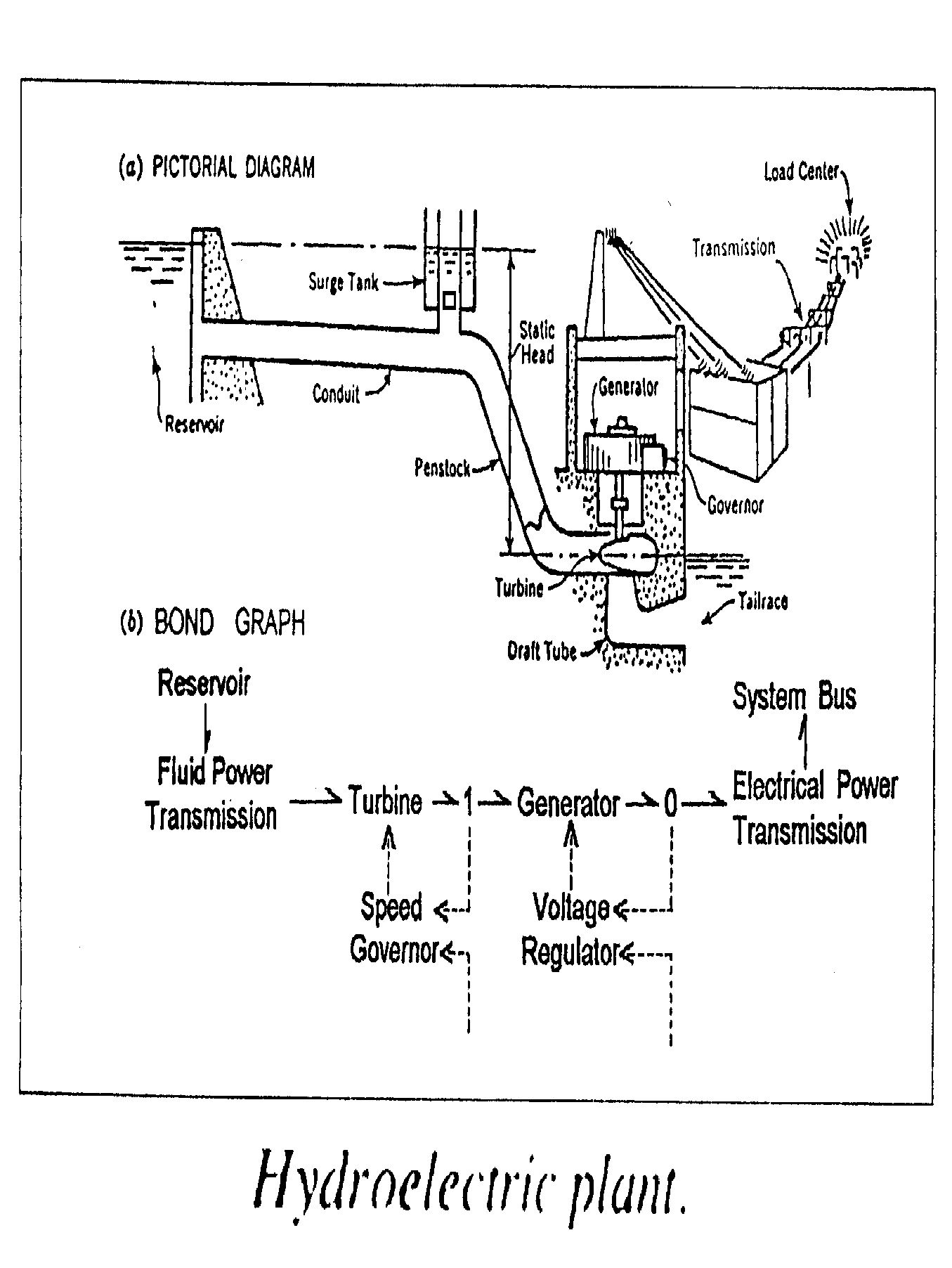
Re: This Week’s Finds in Mathematical Physics (Week 292)
I’m not sure I ever quite got to the bottom of the Legendre/Laplace transform business. Litvonov muddied things further by calling the Legendre transform the idempotent version of the Fourier-Laplace transform here on p. 11.
Perhaps we’ll have the chance to understand some of these issues in terms of your physical systems.