Torsion: Graph Magnitude Homology Meets Combinatorial Topology
Posted by Simon Willerton
.")
As I explained in my previous post, magnitude homology categorifies the magnitude of graphs. There are two questions that will jump out to seasoned students of homology.
- Are there two graphs which have the same magnitude but different homology groups?
- Is there a graph with torsion in its homology groups?
Both of these were stated as open questions by Richard Hepworth and me in our paper as we were unable to answer them, despite thinking about them a fair bit. However, recently both of these have been answered positively!
The first question has been answered positively by Yuzhou Gu in a reply to my post. Well, this is essentially answered, in the sense that he has given two graphs both of which we know (provably) the magnitude of, one of which we know (provably) the magnitude homology groups of and the other of which we can compute the magnitude homology of using mine and James Cranch’s SageMath software. So this just requires verification that the program result is correct! I have no doubt that it is correct though.
The second question on the existence of torsion is what I want to concentrate on in this post. This question has been answered positively by Ryuki Kaneta and Masahiko Yoshinaga in their paper
It is a consequence of what they prove in their paper that the graph below has -torsion in its magnitude homology; SageMath has drawn it as a directed graph, but you can ignore the arrows. (Click on it to see a bigger version.)

In their paper they prove that if you have a finite triangulation of an -dimensional manifold then you can construct a graph so that the reduced homology groups of embed in the magnitude homology groups of :
Following the suggestion in their paper, I’ve taken a minimal triangulation of the real projective plane and used that to construct the above graph. As we know , we know that there is -torsion in .
In the rest of this post I’ll explain the construction of the graph and show explicitly how to give a -torsion class in . I’ll illustrate the theory of Kaneta and Yoshinaga by working through a specific example. Barycentric subdivision plays a key role!
The minimal triangulation of the projective plane
We are going to construct our graph from the minimal triangulation of so let’s have a look at that first. We want to see how the -torsion in the homology of can be expressed using this triangulation as we will need that later for the -torsion in the graph magnitude homology.
The real projective plane can be thought of as the two-sphere quotiented out by the antipodal map. The antipodal map acts on the icosahedral triangulation of the two-sphere. So quotienting the icosahedron by the antipodal map gives us a triangulation of which is in fact the triangulation with fewest simplices. Here is a picture of it.
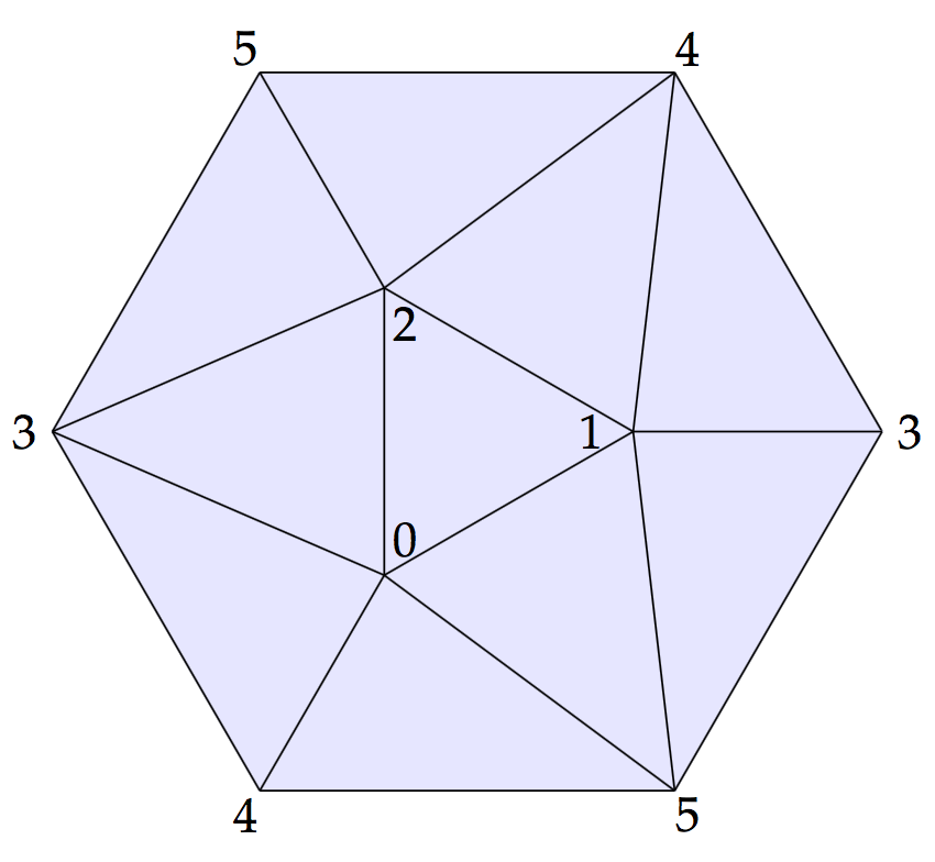
I’ve numbered the vertices and we will label each simplex by its vertices, so is a 2-simplex you can see in the triangulation above. The label for a simplex will have the vertices in linear order.
Let’s recall how we get the -torsion element in homology. If we take the boundary of the ten 2-simplices with the orientation drawn above then we get
(We write rather than because of the orientation conventions which I will gloss over. You can figure them out if you’re interested/concerned. I think they are right!)
As this boundary chain is a cycle. To get homology we quotient cycles out by boundaries, so this cycle is trivial in homology, which means
Thus is a -torsion element. Off the top of my head I can’t think of a nice argument showing that this is non-trivial in homology, but hopefully someone can provide one in the comments! Anyway, we’re going to need this later.
Constructing the graph and the magnitude cycles
Following Kaneta and Yoshinaga, we are now going to use the above triangulation to build our graph . We take the simplices of the triangulation as the nodes of the graph and have an edge if is a facet of , remember that a facet is a face of maximal dimension. We then add top and bottom nodes, so has an arrow to each -simplex and has an arrow from each -dimensional simplex. Here is the graph again. You should be able to see the six vertices, fifteen edges and ten faces of the original triangulation.
A more sophisticated way of saying what we’ve done is the following. The vertices in the triangulation form a poset, the face poset, with the ordering is ‘is a face of’. We add top and bottom elements to that poset. We then take the Hasse diagram which is the graph which has the elements of the poset as its nodes and where there is an edge if but there is no with . Clearly this process gives us a graph from any triangulation of a manifold.
We can obtain the graph in SageMath with a couple of commands:
triangulation = simplicial_complexes.RealProjectivePlane()
poset = triangulation.face_poset().with_bounds()
graph = poset.hasse_diagram()
To see the above picture you can use the following command:
show(poset.plot())
For what we do next it doesn’t matter if we stick with this directed graph or take the associated undirected graph as we are going to be forced to only consider upward pointing edges.
The magnitude chains for this graph
In the previous post I explained that for a finite graph the magnitude chain groups are defined as follows.
A chain generator is a tuple of the form where each is a node of the graph and . The degree is and the length is .
The face map for is defined by:
where means that lies on a shortest path between and , i.e., .
Neither the length nor the endpoints of chains are altered by the face maps, so the magnitude complex splits up into subcomplexes with specified endpoints. So if we define
Then the magnitude chain complex splits as
We will concentrate on the subcomplex of length-four chains from the bottom element to the top element in our graph (here, four is dimension of plus two). Writing and for the bottom and top elements we consider the magnitude chain complex . We will see that the homology of this is isomorphic to and so we get the embedding .
Looking at our graph it is easy to see that a length four chain must be of the form
where is a sequence of simplices, each of which is a face of the following one, in other words it is flag of simplices in our original triangulation. Such a flag can be a full flag like in which each is a facet of the following simplex, or it can be a partial flag like .
Looking at the formula for the face maps you can see that given a generator corresponding to a flag of simplices, each facet of the generator corresponds to a flag with one of the simplices removed.
Those of you familiar with combinatorial topology might have spotted the connection with the barycentric subdivision construction. We will look a little more closely at these flags now.
Barycentric subdivision
One of the things you usually learn in a first course on algebraic topology is that if you have a triangulation of a space then you can form a finer triangulation – the barycentric subdivision – in the following way. Take the midpoint of each simplex in the original triangulation and use these as the vertices of the new triangulation, decomposing each of the old -simplices into new -simplices in ‘the obvious fashion.
For instance, if we take a triangle in our triangulation then each -simplex gets split into new -simplices and the -simplex gets split into new -simplices.
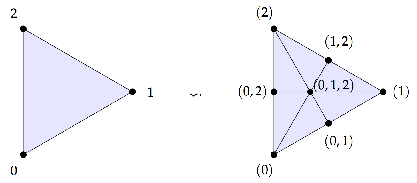
Each new vertex can be labelled by the -simplex that it is the midpoint of. What then is ‘the obvious fashion’ for creating the new simplices? Well each new -simplex in the subdivision corresponds to a flag of old simplices . We can picture the -simplex corresponding to and the -simplex corresponding to as follows.
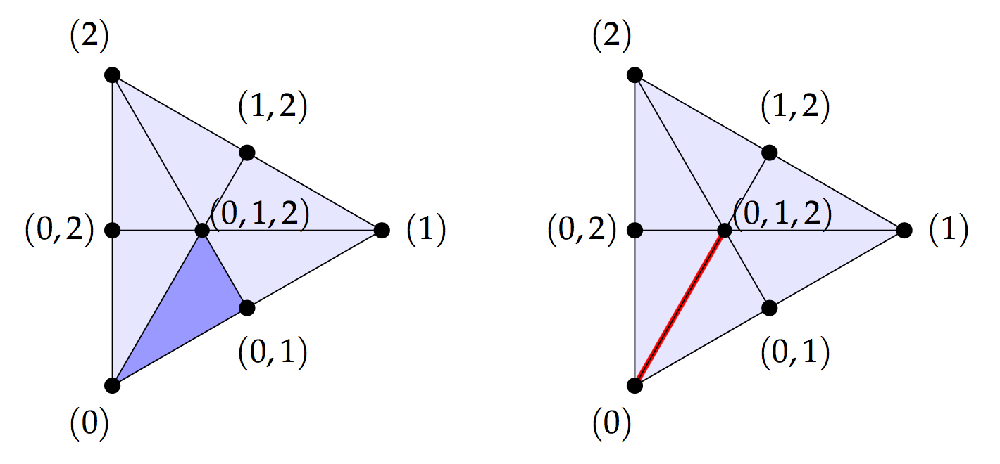
It ought to be clear that for the -simplex in the subdivision corresponding to a flag , each facet corresponds to a flag where one of the old simplices have been removed. So for the facets correspond to , and .
So the barycentric subdivision , as a simplicial complex is isomorphic to the simplicial complex of flags where an -simplex is a flag of simplices of the original triangulation . Well, there’s a subtlety here in that we shouldn’t forget the empty flag! The flags naturally form an augmented simplicial complex, meaning that there is a unique simplex in degree , the empty flag, which is the facet of every -simplex.
So the augmented chain complex , which is obtained from the usual chain complex by sticking a unique generator in degree , is isomorphic to the complex of flags. The homology of the augmented chain complex gives the reduced homology which in practice means you kill off a copy of in degree zero from the usual homology.
The important thing is that we are seeing here precisely the same structure that we saw in the magnitude chain group . We should now make precise.
Synthesis of the two sides: the theorem
I’ve hopefully given the impression that a complex of flags of simplices is isomorphic to both the augmented chain complex of the barycentric subdivision of a triangulation and to a subcomplex of the magnitude chain complex of the graph of the triangulation. Let’s give a proper statement of this now. Kaneta and Yoshinaga have a more general statement in their paper, involving ranked posets rather than just triangulations, but for the purpose of finding torsion, the following will suffice.
Theorem. Suppose that is a finite triangulation of a -manifold , and that is its barycentric subdivision, with the graph obtained as above from the poset structure, then the isomorphism of (augmented) chain groups for
commutes up to sign with the differentials. Thus this induces an isomorphism of homology groups
As a corollary we get that the homology of embeds in the magnitude homology of the graph.
Corollary. With , , and as in the above theorem, the homology of embeds in the magnitude homology of the graph via the following sequence of isomorphisms and embeddings:
The payoff: a torsion element in the homology of our graph
We saw earlier on in this post that
is the non-trivial -torsion element. We can follow this element through the sequence of maps above. We just need to note that the map -chains on to -chains on rewrites each edge as the (signed) sum of its two half-edges, namely
Then we get our non-trivial -torsion element in to be
Thus we have a graph with torsion in its magnitude homology groups!
Re: Torsion: Graph Magnitude Homology Meets Combinatorial Topology
Thanks a lot for explaining (this aspect of) Kaneta and Yoshinaga’s paper, and thanks moreover for making the graph and the torsion class explicit.
Now that there is one example of a graph whose magnitude homology contains torsion, I can’t help wishing for more, especially since the graph constructed above has 33 vertices and 76 edges, which seems pretty big to me.
Q: Is there a graph / metric space which has fewer than 33 vertices / elements and whose magnitude homology has torsion?
One could consider starting with and then deleting or contracting edges to make a smaller graph. You told me by email that deleting edges destroys the torsion property. (Because in some sense this corresponds to puncturing .) But do you know anything about what happens if you contract?
Q: Is there a graph or metric space with torsion in ?