Skip to the Main Content

Note:These pages make extensive use of the latest XHTML and CSS Standards. They ought to look great in any standards-compliant modern browser. Unfortunately, they will probably look horrible in older browsers, like Netscape 4.x and IE 4.x. Moreover, many posts use MathML, which is, currently only supported in Mozilla. My best suggestion (and you will thank me when surfing an ever-increasing number of sites on the web which have been crafted to use the new standards) is to upgrade to the latest version of your browser. If that's not possible, consider moving to the Standards-compliant and open-source Mozilla browser.

March 19, 2018

Magnitude Homology Reading Seminar, I

Posted by Simon Willerton

In Sheffield we have started a reading seminar on the recent paper of Tom Leinster and Mike Shulman Magnitude homology of enriched categories and metric spaces. The plan was to write the talks up as blog posts. Various things, including the massive strike that has been going on in universities in the UK, have meant that I’m somewhat behind with putting the first talk up. The strike also means that we haven’t had many seminars yet!

I gave the first talk which is the one here. It is an introductory talk which just describes the idea of categorification and the paper I wrote with Richard Hepworth on categorifying the magnitude of finite graphs, this is the idea which was generalized by Tom and Mike.

Categorification

Categorification means many things. In this context it is supposed to be the idea of lifting an invariant from taking values in a set to values in a category. Let’s look at two examples.

[This is possibly a caricature of what actually happened. It would be nice to have some references!] In the eighteenth century, mathematicians such as Riemann knew about the Euler characteristic of surfaces (and possibly manifolds). This is a fundamental invariant which seems to crop up in all sorts of places. Towards the end of the century Poincar'e introduced homology groups H (M)\text{H}_\star(M) of a manifold MM and was aware

χ(M)=rank(H (M))= i(1) irank(H i(M)). \chi(M)=rank(\text{H}_\star(M))= \sum_i (-1)^i rank (\text{H}_i(M)).

I get the impression the functorial nature of homology was not appreciated until later, but this adds another layer of structure.

Around 1985 Jones introduced his eponymous polynomial J(L)[q ±1]\text{J}(L)\in \mathbb{Z}[q^{\pm 1}] for a knot or link LL in 33-space. This gives a polynomial invariant of links. In around 1999, Khovanov introduced Khovanov homology Kh ,(L)Kh_{\star, \star}(L) for a link LL, this is bigraded group. The Jones polynomial is obtained from it by taking the dimension (or Euler characteristic!) in an appropriate graded sense:

J(L)= i,j(1) iq jrank(Kh i,j(L)). \text{J}(L)= \sum_{i,j} (-1)^i q^j rank( Kh_{i,j}(L)).

In both these cases we lift an invariant which takes values in a set (either \mathbb{Z} or [q ±1] \mathbb{Z}[q^{\pm 1}]) to an invariant which takes values in a category (either graded groups or bigraded groups). This lifted invariant has a richer structure and functorial properties, but is probably harder to calculate! This is what we mean by categorifying an invariant.

Magnitude of enriched categories

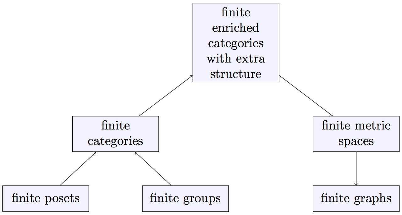
There was a classical notion of Euler characteristic for finite groups and also one for finite posets. We know that finite groups and finite posets are both examples of finite categories (at one extreme with only one object and at the other extreme with at most one morphism between each pair of objects). Tom found a common generalization of these Euler characteristics which is the idea of an Euler characteristic for finite categories (we will see the definition next week). He further generalized that to the notion of an Euler characteristic for enriched categories (with a additional bit of structure, wait for next week). Finite metric spaces are examples of enriched categories and so have a notion of Euler characteristic. We decided the name was too confusing so after consulting a thesaurus we decided on “magnitude” (having toyed with the name “cardinality”). Tom later noticed something nice about the magnitude of the metric spaces that you get from finite graphs (partly because these have integer-valued metrics).

The journey from the Euler characteristics of finite posets and finite groups to the magnitude of finite graphs via a sequence of generalizations and specializations can be viewed as a trip up and then down the following picture.

hierarchy of some category enrichments

Magnitude of metric spaces (more next week)

For X={x 1,x n}X=\{x_1,\dots x_n\} a finite metric space with the metric we can define a matrix ZZ by Z i,j=e d(x i,x j)Z_{i,j}=e^{-\text{d}(x_i,x_j)}. The magnitude |X||X| is defined to be the sum of the entries of the inverse matrix (if it exists): |X|:= i,j(Z 1) i,j|X|:=\sum_{i,j}(Z^{-1})_{i,j}. It is actually more interesting if we look at what happens as we scale XX (or perhaps if we introduce an indeterminate into the metric). For t>0t> 0, we define tXt\cdot X to have the same underlying set, but with the metric scaled by a factor of tt. This gives us the magnitude function |tX|\left|t\cdot X\right| which is a function of tt.

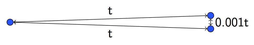
We can have a look at a simple example where we take XX to be a three-point metric space in which two points are much, much closer to each other than they are to the third point. Here is a picture of tXt\cdot X.

mh_sem_1_three_points.png

Here is the graph of the magnitude function of the metric space XX.

graph of the magnitude function

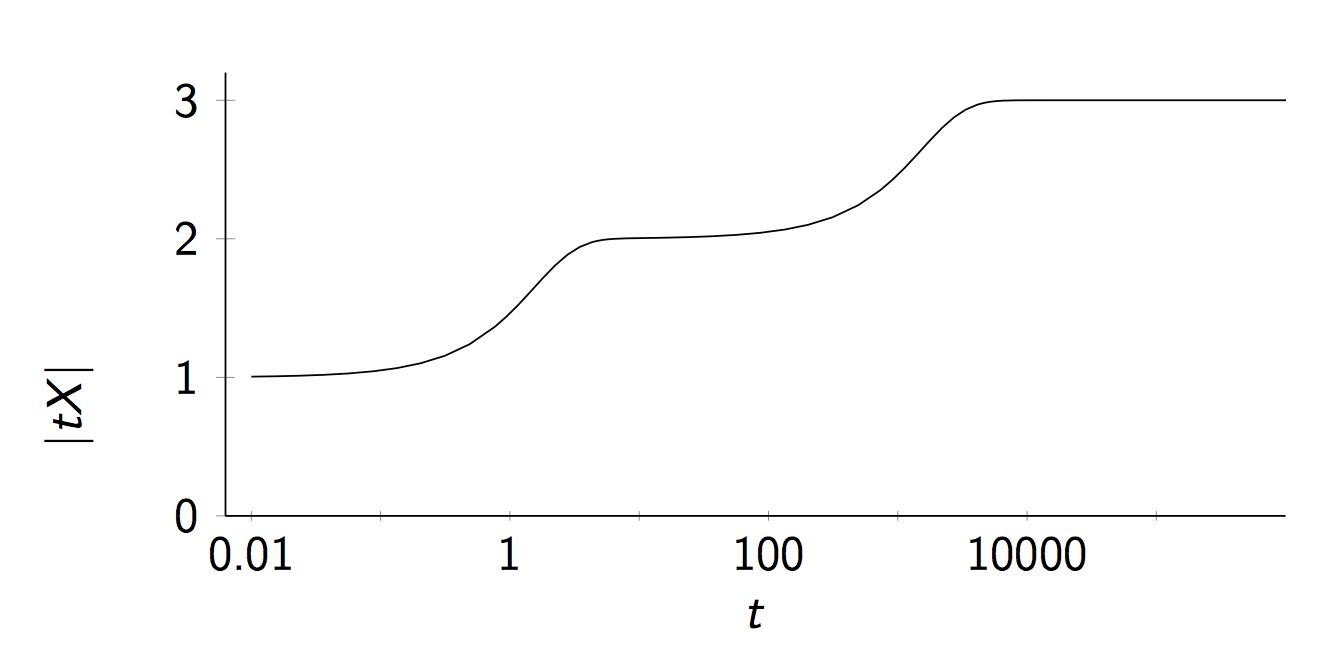
This shows in some sense how the magnitude can be viewed as an “effective number of points”. At small scales there is effectively one point, at middling scales there is effectively two points and at very large scales there are effectively three points.

Although the definition looks rather ad hoc, it turns out that it has various connections to thinks like measurements of biodiversity, Hausdorff dimension, volumes, potential theory and several other fun things.

Magnitude of graphs

Suppose that GG is a finite graph, then it gives rise to a finite metric space (which we will also write as GG) which has the vertices of GG as its points and the shortest path distance as its metric, where all edges have length one.

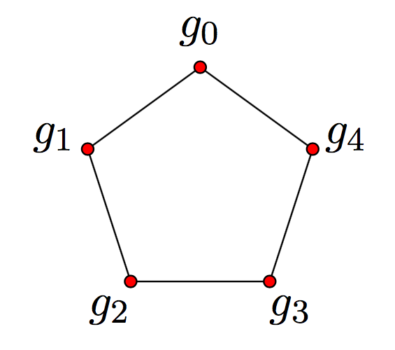
For example we have the five-cycle graph below with d(g 0,g 3)=2\text{d}(g_0, g_3)=2.

mh_sem_1_five_cycle_graph.png

Tom noticed that we can use the magnitude function of the associated metric space to get an integral power series from the graph. Firstly, we can write q=e tq=e^{-t} then the entries of the matrix ZZ are just integer powers of qq as all of the distances in GG are integral. This means that the entries of Z 1Z^{-1} are just rational functions of qq (with integer coefficients) and hence so is their sum, the magnitude function. Moreover the denominator of this rational function is the determinant of ZZ which, as the diagonal entries of ZZ are all e 0e^{0}, i.e., 11, is of the form 1+powers of q1+\text{powers of }q. So we can take a power series expansion of |tG||t\cdot G| to get an integer power series in q=e tq=e^{-t}. We denote this power series by #G\# G.

For example, for the five-cycle graph C 5C_5 pictured above we have

#C 5=510q+10q 220q 4+40q 540q 6+. \# C_5 = 5-10q+10q^2-20q^4+40q^5-40q^6+\cdots.

In general we can identify the first two coefficients as the number of vertices and 2-2 times the number of edges, respectively.

Categorifying the magnitude of graphs

As Richard Hepworth noticed, we can categorify this! In other words, we can find a homology theory which has the magnitude power series #GZ[q]\# G\in \Z[q] as its graded Euler characteristic.

For a finite graph GG define the magnitude chain groups as follows.

MC k,l(G)=(x 0,,x k)|x i1x i,dd(x i1,x i)=l. MC_{k,l}(G)=\left\langle (x_0,\dots, x_k) \big | x_{i-1}\ne x_{i},\quad \sum \dd(x_{i-1}, x_i)=l\right\rangle.

For example a chain group generator for the five-cycle graph from above is (g 0,g 1,g 2,g 4,g 2)MC 4,6(C 5)(g_0, g_1, g_2, g_4, g_2)\in MC_{4,6}(C_5).

We define maps i:MC k,l(G)MC k1,l(G)\partial_i\colon MC_{k,l}(G)\to MC_{k-1,l}(G) for i=1,,k1i=1,\dots, k-1:

i(x 0,,x k)={(x 0,,x i^,,x k) ifx i1<x i<x i+1, 0 otherwise. \partial_{i}(x_0,\ldots,x_k) = \begin{cases} (x_0,\ldots,\widehat{x_i},\ldots,x_k) & \text{if}\,\, x_{i-1}&lt;x_{i}&lt;x_{i+1}, \\ 0 & \text{otherwise}. \end{cases}

where x i1<x i<x i+1x_{i-1}&lt;x_{i}&lt;x_{i+1} means that x ix_i lies on a shortest path between x i1x_{i-1} and x i+1x_{i+1}, i.e., d(x i1,x i)+d(x i,x i+1)=d(x i1,x i+1)\text{d}(x_{i-1},x_i)+\text{d}(x_i,x_{i+1})=\text{d}(x_{i-1},x_{i+1}).

So for our example chain generator in C 5C_5 you can check that we have

i(g 0,g 1,g 2,g 4,g 2)={(g 0,g 2,g 4,g 2) ifi=1, 0 otherwise. \partial_{i}(g_0, g_1, g_2, g_4, g_2) = \begin{cases} (g_0, g_2, g_4, g_2) & \text{if}\,\, i=1, \\ 0 & {otherwise}. \end{cases}

In the usual way, the differential :MC k,l(G)MC k1,l(G)\partial\colon MC_{k,l}(G)\to MC_{k-1,l}(G) is defined as the alternating sum

= 1 2++(1) k1 k1. \partial=\partial_1-\partial_2+\cdots+(-1)^{k-1}\partial_{k-1}.

One can show that this is a differential, so that =0\partial\circ\partial =0. Then taking homology gives what is defined to be magnitude homology groups of the graph:

MH k,l(G)=H k(MC *,l(G),). \MH_{k,l}(G)= \text{H}_k(\MC_{\ast,l}(G), \partial).

By direct computation you can calculate the ranks of the magnitude homology groups of the five-cycle graph. The following table shows the ranks rank(MH k,l(C 5))rank(MH_{k,l}(C_5)) for small kk and ll.

k 0 1 2 3 4 5 6 χ(MH *,l(C 5)) 0 5 5 1 10 10 2 10 10 l 3 10 10 0 4 30 10 20 5 50 10 40 6 20 70 10 40 \begin{array}{rrrrrrrrrrc} &&&&&k\\ &&0&1&2&3&4&5&6&&\chi(MH_{\ast,l}(C_5))\\ &0 & 5&&&&&&&\qquad&5\\ & 1 & & 10 &&&&&&&-10 \\ &2 & && 10 &&&&&&10\\ l& 3 &&& 10 & 10 &&&&&0 \\ & 4 &&&& 30 & 10 &&&&-20\\ & 5 &&&&& 50 & 10 &&&40 \\ & 6 &&&&& 20 & 70 & 10 &&-40 \end{array}

The final column shows the Euler characteristics, which are just the alternating sums of entries in the rows. You can check that these are precisely the coefficients in the power series #C 5\# C_5 given above: this illustrates the fact that graph magnitude homology does indeed categorify graph magnitude in the sense of the following theorem.

Theorem #G= k,l0(1) kq lrank(MH k,l(G))[[q]]. \#G = \sum_{k,l\geq 0} (-1)^k q^l \,rank \bigl(MH_{k,l}(G)\bigr)\in \mathbb{Z}[[q]].

Thus we have MH *,*MH_{\ast,\ast} which a bigraded group valued invariant of graphs which is functorial with respect to certain maps of graphs and has properties like Kunneth Theorem and long exact sequences: richer but harder to calculate than the graph magnitude.

In the following weeks we will hopefully see how Mike and Tom have generalized this construction up to the top of the picture above, namely to certain enriched categories with extra structure.

Posted at March 19, 2018 8:59 AM UTC

TrackBack URL for this Entry:   https://golem.ph.utexas.edu/cgi-bin/MT-3.0/dxy-tb.fcgi/3028

14 Comments & 0 Trackbacks

Re: Magnitude Homology Reading Seminar, I

[This is possibly a caricature of what actually happened. It would be nice to have some references!]

This paper by Colin McLarty might be a good place to start, at least for the earlier parts of the story.

Posted by: Mark Meckes on March 19, 2018 2:36 PM | Permalink | Reply to this

Re: Magnitude Homology Reading Seminar, I

Thanks Mark, I’ll have a look!

Posted by: Simon Willerton on March 19, 2018 4:53 PM | Permalink | Reply to this

Re: Magnitude Homology Reading Seminar, I

The link to Hepworth-Willerton is incorrect.

Posted by: Yuzhou Gu on March 19, 2018 4:35 PM | Permalink | Reply to this

Re: Magnitude Homology Reading Seminar, I

Fixed! Thank you.

Posted by: Simon Willerton on March 19, 2018 4:54 PM | Permalink | Reply to this

Re: Magnitude Homology Reading Seminar, I

I am not sure this is the correct place but let me say some observations/results on magnitude homology of graphs.

  1. Hepworth-Willerton asked whether there are graphs with same magnitude but different magnitude homology. Note that magnitude is computable in polynomial time but it is not obvious we can do so with magnitude homology. So hard graph isomorphism instances should suffice. Specifically, we can take the two graphs to be rook (4,4) graph and Shrikhande graph.

  2. Calculations of magnitude homology can often be done using algebraic Morse theory (Jollenbeck 05, Skoldberg 06).

Let me give an example for odd cyclic graphs C 2m+1C_{2m+1}. Fixing a start point, any sequence of points (x 0,x 1,,x k)(x_0,x_1,\ldots,x_k) can be written as a sequence of numbers (a 1,,a k)(a_1,\ldots,a_k) in {m,,1,1,,m}\{-m,\ldots,-1, 1, \ldots,m\}, where a i=x ix i1(mod(2m+1))a_i = x_i-x_{i-1} \pmod{(2m+1)}. Deleting a point in the sequence is sequence is equivalent to merging to adjacent numbers. Two numbers can be merged if and only if (1) their signs are equal and (2) absolute value of their sum is m\le m.

Using some tensor product decomposition we can reduce the problem to computing the homology of the chain complex generated by sequences only with positive numbers. The morse matching is: (,k,m,1,,m,1)(\cdots, k,m,1,\ldots,m,1)-(,k1,1,m,1,,m,1)(\cdots,k-1,1,m,1,\ldots,m,1) for 2km2\le k\le m and any prefix. The remaining elements are of the form (1,m,1,,m,1)(1,m,1,\ldots,m,1) and (m,1,,m,1)(m,1,\ldots,m,1).

For even cyclic graphs we can also compute magnitude homology using algebraic morse theory, but it is more complicated. (Results for cyclic graphs match predictions made in Hepworth-Willerton.) I also tried for some time proving Whitney twist, but did not succeed.

Posted by: Yuzhou Gu on March 19, 2018 6:04 PM | Permalink | Reply to this

Re: Magnitude Homology Reading Seminar, I

Yuzhou, that sounds great. Are you planning on writing this up?

I don’t quite follow the reasoning in (1) probably because I don’t know anything about the hard isomorphism problem, and I don’t know anything about algebraic Morse theory in (2); so it would be nice to hear more about this.

I can, however, give some verification of your two graphs with the same magnitude but different magnitude homology groups.

Let’s start with the 4×44\times 4 rook graph, R 4,4R_{4,4}. This is isomorphic to the Cartesian product K 4K 4K_4\square K_4 where K 4K_4 is the complete graph on four vertices. An easy computation (eg. by Speyer’s homogeneous magnitude formula) gives the magnitude function of this complete graph:

|K 4|=41+3q.|K_4|=\frac{4}{1+3q}.

So by Tom’s multiplicativity result for the Cartesian product we have

|R 4,4|=|K 4K 4|=|K 4||K 4|=169q 2+6q+1.|R_{4,4}|= |K_4\square K_4| = |K_4|\cdot |K_4| = \frac{16}{9q^2 + 6q + 1}.

On the other hand, a quick check with SageMath, using the command graphs.ShrikhandeGraph().magnitude_function() gives the same answer for the Shrikhande graph, SS:

|S|=169q 2+6q+1.|S|= \frac{16}{9q^2 + 6q + 1}.

So we do indeed have |S|=|R 4,4||S| = |R_{4,4}|. Taking the power series expansions gives us

#S=#R 4,4 = i=0 16(i+1)(3q) i =1696q+432q 21728q 3+6480q 423328q 5+. \begin{aligned} \# S = \# R_{4,4} &= \sum_{i=0}^\infty 16 (i+1)(-3q)^i \\ &= 16 - 96q + 432q^2 - 1728q^3 +6480q^4 - 23328q^5 +\dots\,. \end{aligned}

Now for the magnitude homology. Let’s do the rooks graph first. From the result in mine and Richard’s paper we know that for the complete graph the magnitude homology MH *,*(K 4)MH_{\ast,\ast}(K_4) is torsion-free and diagonal (where ‘diagonal’ means that the only non-trivial groups are MH k,k(K 4)MH_{k,k}(K_4)). Our Kunneth theorem then implies that R 4,4=K 4K 4R_{4,4} = K_4\square K_4 is also diagonal and torsion-free, so from the above magnitude expansion we have that in low degree MH k,l(R 4,4)MH_{k,l}(R_{4,4}) has rank as follows.

k 0 1 2 3 4 5 0: 16 1: 96 2: 432 l3: 1728 4: 6480 5: 23328 \begin{array}{rrrrrrr} & & & & k\\ & 0 & 1& 2& 3 & 4& 5\\ 0:& 16 & & & & & \\ 1:& & 96 & & & & \\ 2:& & & 432 & & & \\ l\,\,\, 3:& & & & 1728 & & \\ 4:& & & & & 6480 & \\ 5:& & & & & & 23328 \end{array}

Now for the Shrikande graph. A computation in SageMath for the Shrikhande graph gives us that, over the rationals, MH k,l(S)MH_{k,l}(S) has the following rank:

k 0 1 2 3 4 5 0: 16 1: 96 2: 432 l3: 1728 4: 144 6624 5: 1632 24960 \begin{array}{rrrrrrr} & & & & k\\ & 0 & 1& 2& 3 & 4& 5\\ 0:& 16 & & & & & \\ 1:& & 96 & & & & \\ 2:& & & 432 & & & \\ l\,\,\, 3:& & & & 1728 & & \\ 4:& & & & 144 & 6624 & \\ 5:& & & & & 1632 & 24960 \end{array}

Excellent! Different magnitude homology, as you said.

Posted by: Simon Willerton on March 20, 2018 1:07 PM | Permalink | Reply to this

Re: Magnitude Homology Reading Seminar, I

Oh, “hard graph isomorphism instances should suffice” is not a theorem, but an idea of how we can generate graphs that are indistinguishable using magnitude but distinguishable using magnitude homology. Hard graph isomorphism instances mean two graphs that are (possibly) difficult to distinguish using polynomial-time algorithms. So magnitude, which is computable in polynomial time, probably cannot distinguish these two graphs. That magnitude homology can distinguish them is just a hope, since magnitude homology is so strong. So yes, this is not rigorous reasoning. Anyway this gives graphs we want.

I may write this up in May or June, when the school term ends.

If you want to learn about algebraic Morse theory, you can refer to Skoldberg, Morse theory from an algebraic viewpoint; or for a very quick introduction, refer to Section 1.1 of Lampret, Vavpetic, (Co)homology of Lie algebras via algebraic Morse theory.

Posted by: Yuzhou Gu on March 20, 2018 5:01 PM | Permalink | Reply to this

Re: Magnitude Homology Reading Seminar, I

Splendid.

Can I ask how you proved that the magnitude homology of the two graphs are different? And did you come up with a list of potential candidates using hard graph isomorphism instances and then try them, or was this the first pair you tried?

Posted by: Simon Willerton on March 20, 2018 8:52 PM | Permalink | Reply to this

Re: Magnitude Homology Reading Seminar, I

was this the first pair you tried?

Wikipedia rook graph does say

When n=4n = 4, there is another strongly regular graph, the Shrikhande graph, with the same parameters as the 4×44\times 4 rook’s graph. The Shrikhande graph obeys the same properties listed by Moon and Moser.

So I guess their similarity is well known by those who know such things.

Posted by: RodMcGuire on March 20, 2018 10:56 PM | Permalink | Reply to this

Re: Magnitude Homology Reading Seminar, I

To your disappointment, I verified that using code provided at arXiv. (On the other hand, the proof that their magnitude are the same is slightly simpler than yours: observe that both graphs are vertex-transitive and then use Speyer’s formula.)

This pair is the first pair I tried. I just tried another pair: Dodecahedral graph and Desargues graph, and it worked. (The hardest part is to find two vertex-transitive graphs such that the multisets {d(g,v):vV}\{d(g,v): v\in V\} are the same.) Magnitude homology indeed does well in distinguishing graphs.

Posted by: Yuzhou Gu on March 20, 2018 11:20 PM | Permalink | Reply to this

Re: Magnitude Homology Reading Seminar, I

Cool! These are exciting developments.

Posted by: Tom Leinster on March 21, 2018 4:34 PM | Permalink | Reply to this

Re: Magnitude Homology Reading Seminar, I

Simon wrote:

Towards the end of the century Poincaré introduced homology group H *(M)H_*(M) of a manifold MM

I’ve looked at his Analysis Situs and I don’t remember anything about homology groups, just Betti numbers and perhaps other numerical invariants associated to what we’d now call the torsion part of the homology groups. I think it was Emmy Noether who explicitly introduced homology groups, though in retrospect we can find them lurking in earlier work — indeed, we can scarcely understand earlier work without thinking about homology groups! So I’d say Noether categorified earlier work, by treating Betti numbers as ranks of homology groups. This set the stage for mathematicians to study the effect of maps on homology, which in turn led Eilenberg and Mac Lane to invent ‘functors’.

Here’s what I said in a talk on The Rise and Spread of Algebraic Topology:

We now say the iith Betti number of a topological space XX is the rank of H i(X)H_i(X). But that’s not what Enrico Betti said!

Betti defined his numbers in 1871. In 1895 Poincaré recalled them in his Analysis Situs. In what would later be seen as a massive understatement, he wrote:

Meanwhile, the field is by no means exhausted.

Poincaré said what it means for two oriented submanifolds of a manifold XX to be homologous. He showed how to add and subtract homology classes. He essentially said that the iith Betti number of XX is β i\beta_i if XX has at most β i\beta_i linearly independent homology classes of ii-dimensional submanifolds.

Only 20 years later, in 1915, did Alexander prove that Betti numbers are topological invariants.

In the summers of 1926–1928, Alexandroff and Hopf lectured on algebraic topology in Goettingen. Emmy Noether attended and pointed out that iith Betti number is the rank of an abelian group

H i(X)=ker iim i+1 H_i(X) = \displaystyle{ \frac{\ker \partial_i}{\im \, \partial_{i+1}} }

where

i:C i(X)C i1(X) \partial_i : C_i(X) \to C_{i-1}(X)

is a map between ‘chain groups’. She also noticed that a map of simplicial complexes induced a map of homology groups. All this was new!

Noether never published a single paper about these ideas, and they spread slowly.

All these ideas were a very long time in the making because the people doing homology and homotopy theory were not algebraists and the algebraists didn’t take any interest. The only person who took any interest was Emmy Noether.Peter Hilton

Posted by: John Baez on March 24, 2018 7:50 AM | Permalink | Reply to this

Re: Magnitude Homology Reading Seminar, I

Based on a cursory reading of the paper by Colin McLarty I linked to above, and some of its references, it seems that some people (including Mac Lane and McLarty) contend that Poincaré understood perfectly well that in his adding and subtracting of homology classes amounted to working with groups, but that for reasons I don’t find very clear, Poincaré avoided using the term “group” in this context. Others (notably Dieudonné) disagree. (McLarty also claims that Lefschetz used the term “homology group” before Noether did.)

Of course, no one disputes the central role that Noether played in creating homology theory in its modern form. McLarty’s focus is in particular on how Noether set the stage for the invention of functors.

Posted by: Mark Meckes on March 24, 2018 5:54 PM | Permalink | Reply to this

Re: Magnitude Homology Reading Seminar, I

Here is an email exchange I had with Tom Leinster about using Lawvere balls in an enriched category to define persistant homology of a suitable enriched category. As it turns out the two things are related.

Hi Tom,

This post on MathOverflow has got me thinking. If we can define open balls in any suitable enriched category, then why not try and apply some ideas from persistant homology?

Persistant homology is the process of taking a set of points of a metric space and studying the homology groups of the Vietoris-Rips complex for some small parameter E, and seeing which groups persist when E is varied. It has some interesting applications in topological data analysis.

I find this interesting because metric spaces can be generalised very naturally to an enriched category theory setting. And a categorical Vietoris-Rips could associate a homotopy type to a V-enriched category C, for each object in V.

Now I have answered the question I linked, where I reference a paper by Lawvere: Taking categories seriously. So if we have some V-enriched category C, we can consider any small full subcategory and call this our point cloud. We can then build up a simplicial complex by considering the Lawvere balls at each element, this can be made more sturdy if we also associate an ordering to the objects of our point cloud. What should be left is a simplicial complex representing the category.

The reason for this email is because I know you have thought some bit about metric spaces categorically.

I would love to know your thoughts and feelings about such a concept.

Thanks,

Ali Caglayan

And his reply:

Hi Ali,

Interesting question! I don’t think I have anything interesting to say about it at the moment, but we’ve had some discussions about homology of categories at the n-Category Cafe recently -

magnitude reading seminar I

magnitude reading seminar II

so you might consider posting your email as a comment there. All that stuff is about magnitude homology rather than persistent homology, but it’s been shown recently by Nina Otter that the two things are related (https://arxiv.org/abs/1807.01540), so your idea wouldn’t be out of place on those posts.

All the best,

Tom

Posted by: Ali Caglayan on September 18, 2018 5:13 PM | Permalink | Reply to this

Post a New Comment