Skip to the Main Content

Note:These pages make extensive use of the latest XHTML and CSS Standards. They ought to look great in any standards-compliant modern browser. Unfortunately, they will probably look horrible in older browsers, like Netscape 4.x and IE 4.x. Moreover, many posts use MathML, which is, currently only supported in Mozilla. My best suggestion (and you will thank me when surfing an ever-increasing number of sites on the web which have been crafted to use the new standards) is to upgrade to the latest version of your browser. If that's not possible, consider moving to the Standards-compliant and open-source Mozilla browser.

June 11, 2016

How the Simplex is a Vector Space

Posted by Tom Leinster

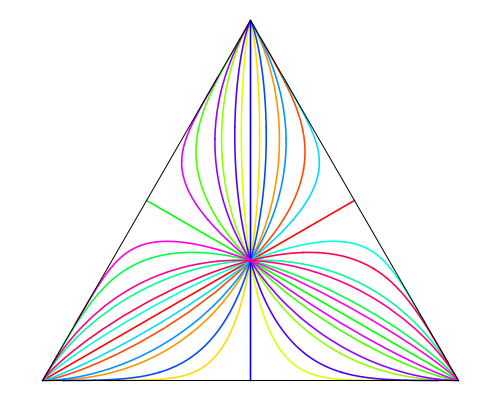
It’s an underappreciated fact that the interior of every simplex Δ n\Delta^n is a real vector space in a natural way. For instance, here’s the 2-simplex with twelve of its 1-dimensional linear subspaces drawn in:

Triangle with some curves

(That’s just a sketch. See below for an accurate diagram by Greg Egan.)

In this post, I’ll explain what this vector space structure is and why everyone who’s ever taken a course on thermodynamics knows about it, at least partially, even if they don’t know they do.

Let’s begin with the most ordinary vector space of all, n\mathbb{R}^n. (By “vector space” I’ll always mean vector space over \mathbb{R}.) There’s a bijection

(0,) \mathbb{R} \leftrightarrow (0, \infty)

between the real line and the positive half-line, given by exponential in one direction and log in the other. Doing this bijection in each coordinate gives a bijection

n(0,) n. \mathbb{R}^n \leftrightarrow (0, \infty)^n.

So, if we transport the vector space structure of n\mathbb{R}^n along this bijection, we’ll produce a vector space structure on (0,) n(0, \infty)^n. This new vector space (0,) n(0, \infty)^n is isomorphic to n\mathbb{R}^n, by definition.

Explicitly, the “addition” of the vector space (0,) n(0, \infty)^n is coordinatewise multiplication, the “zero” vector is (1,,1)(1, \ldots, 1), and “subtraction” is coordinatewise division. The scalar “multiplication” is given by powers: multiplying a vector y=(y 1,,y n)(0,) n\mathbf{y} = (y_1, \ldots, y_n) \in (0, \infty)^n by a scalar λ\lambda \in \mathbb{R} gives (y 1 λ,,y n λ)(y_1^\lambda, \ldots, y_n^\lambda).

Now, the ordinary vector space n\mathbb{R}^n has a linear subspace UU spanned by (1,,1)(1, \ldots, 1). That is,

U={(λ,,λ):λ}. U = \{(\lambda, \ldots, \lambda) \colon \lambda \in \mathbb{R} \}.

Since the vector spaces n\mathbb{R}^n and (0,) n(0, \infty)^n are isomorphic, there’s a corresponding subspace WW of (0,) n(0, \infty)^n, and it’s given by

W={(e λ,,e λ):λ}={(γ,,γ):γ(0,)}. W = \{(e^\lambda, \ldots, e^\lambda) \colon \lambda \in \mathbb{R} \} = \{(\gamma, \ldots, \gamma) \colon \gamma \in (0, \infty)\}.

But whenever we have a linear subspace of a vector space, we can form the quotient. Let’s do this with the subspace WW of (0,) n(0, \infty)^n. What does the quotient (0,) n/W(0, \infty)^n/W look like?

Well, two vectors y,z(0,) n\mathbf{y}, \mathbf{z} \in (0, \infty)^n represent the same element of (0,) n/W(0, \infty)^n/W if and only if their “difference” — in the vector space sense — belongs to WW. Since “difference” or “subtraction” in the vector space (0,) n(0, \infty)^n is coordinatewise division, this just means that

y 1z 1=y 2z 2==y nz n. \frac{y_1}{z_1} = \frac{y_2}{z_2} = \cdots = \frac{y_n}{z_n}.

So, the elements of (0,) n/W(0, \infty)^n/W are the equivalence classes of nn-tuples of positive reals, with two tuples considered equivalent if they’re the same up to rescaling.

Now here’s the crucial part: it’s natural to normalize everything to sum to 11. In other words, in each equivalence class, we single out the unique tuple (y 1,,y n)(y_1, \ldots, y_n) such that y 1++y n=1y_1 + \cdots + y_n = 1. This gives a bijection

(0,) n/WΔ n (0, \infty)^n/W \leftrightarrow \Delta_n^\circ

where Δ n \Delta_n^\circ is the interior of the (n1)(n - 1)-simplex:

Δ n ={(p 1,,p n):p i>0,p i=1}. \Delta_n^\circ = \{(p_1, \ldots, p_n) \colon p_i \gt 0, \sum p_i = 1 \}.

You can think of Δ n \Delta_n^\circ as the set of probability distributions on an nn-element set that satisfy Cromwell’s rule: zero probabilities are forbidden. (Or as Cromwell put it, “I beseech you, in the bowels of Christ, think it possible that you may be mistaken.”)

Transporting the vector space structure of (0,) n/W(0, \infty)^n/W along this bijection gives a vector space structure to Δ n \Delta_n^\circ. And that’s the vector space structure on the simplex.

So what are these vector space operations on the simplex, in concrete terms? They’re given by the same operations in (0,) n(0, \infty)^n, followed by normalization. So, the “sum” of two probability distributions p\mathbf{p} and q\mathbf{q} is

(p 1q 1,p 2q 2,,p nq n)p 1q 1+p 2q 2++p nq n, \frac{(p_1 q_1, p_2 q_2, \ldots, p_n q_n)}{p_1 q_1 + p_2 q_2 + \cdots + p_n q_n},

the “zero” vector is the uniform distribution

(1,1,,1)1+1++1=(1/n,1/n,,1/n), \frac{(1, 1, \ldots, 1)}{1 + 1 + \cdots + 1} = (1/n, 1/n, \ldots, 1/n),

and “multiplying” a probability distribution p\mathbf{p} by a scalar λ\lambda \in \mathbb{R} gives

(p 1 λ,p 2 λ,,p n λ)p 1 λ+p 2 λ++p n λ. \frac{(p_1^\lambda, p_2^\lambda, \ldots, p_n^\lambda)}{p_1^\lambda + p_2^\lambda + \cdots + p_n^\lambda}.

For instance, let’s think about the scalar “multiples” of

p=(0.2,0.3,0.5)Δ 3. \mathbf{p} = (0.2, 0.3, 0.5) \in \Delta_3.

“Multiplying” p\mathbf{p} by λ\lambda \in \mathbb{R} gives

(0.2 λ,0.3 λ,0.5 λ)0.2 λ+0.3 λ+0.5 λ \frac{(0.2^\lambda, 0.3^\lambda, 0.5^\lambda)}{0.2^\lambda + 0.3^\lambda + 0.5^\lambda}

which I’ll call p (λ)\mathbf{p}^{(\lambda)}, to avoid the confusion that would be created by calling it λp\lambda\mathbf{p}.

When λ=0\lambda = 0,   p (λ)\mathbf{p}^{(\lambda)} is just the uniform distribution (1/3,1/3,1/3)(1/3, 1/3, 1/3) — which of course it has to be, since multiplying any vector by the scalar 00 has to give the zero vector.

For equally obvious reasons, p (1)\mathbf{p}^{(1)} has to be just p\mathbf{p}.

When λ\lambda is large and positive, the powers of 0.50.5 dominate over the powers of the smaller numbers 0.20.2 and 0.30.3, so p (λ)(0,0,1)\mathbf{p}^{(\lambda)} \to (0, 0, 1) as λ\lambda \to \infty.

For similar reasons, p (λ)(1,0,0)\mathbf{p}^{(\lambda)} \to (1, 0, 0) as λ\lambda \to -\infty. This behaviour as λ±\lambda \to \pm\infty is the reason why, in the picture above, you see the curves curling in at the ends towards the triangle’s corners.

Some physicists refer to the distributions p (λ)\mathbf{p}^{(\lambda)} as the “escort distributions” of p\mathbf{p}. And in fact, the scalar multiplication of the vector space structure on the simplex is a key part of the solution of a very basic problem in thermodynamics — so basic that even I know it.

The problem goes like this. First I’ll state it using the notation above, then afterwards I’ll translate it back into terms that physicists usually use.

Fix ξ 1,,ξ n,ξ>0\xi_1, \ldots, \xi_n, \xi \gt 0. Among all probability distributions (p 1,,p n)(p_1, \ldots, p_n) satisfying the constraint

ξ 1 p 1ξ 2 p 2ξ n p n=ξ, \xi_1^{p_1} \xi_2^{p_2} \cdots \xi_n^{p_n} = \xi,

which one minimizes the quantity

p 1 p 1p 2 p 2p n p n? p_1^{p_1} p_2^{p_2} \cdots p_n^{p_n}?

It makes no difference to this question if ξ 1,,ξ n,ξ\xi_1, \ldots, \xi_n, \xi are normalized so that ξ 1++ξ n=1\xi_1 + \cdots + \xi_n = 1 (since multiplying each of ξ 1,,ξ n,ξ\xi_1, \ldots, \xi_n, \xi by a constant doesn’t change the constraint). So, let’s assume this has been done.

Then the answer to the question turns out to be: the minimizing distribution p\mathbf{p} is a scalar multiple of (ξ 1,,ξ n)(\xi_1, \ldots, \xi_n) in the vector space structure on the simplex. In other words, it’s an escort distribution of (ξ 1,,ξ n)(\xi_1, \ldots, \xi_n). Or in other words still, it’s an element of the linear subspace of Δ n \Delta_n^\circ spanned by (ξ 1,,ξ n)(\xi_1, \ldots, \xi_n). Which one? The unique one such that the constraint is satisfied.

Proving that this is the answer is a simple exercise in calculus, e.g. using Lagrange multipliers.

For instance, take (ξ 1,ξ 2,ξ 3)=(0.2,0.3,0.5)(\xi_1, \xi_2, \xi_3) = (0.2, 0.3, 0.5) and ξ=0.4\xi = 0.4. Among all distributions (p 1,p 2,p 3)(p_1, p_2, p_3) that satisfy the constraint

0.2 p 1×0.3 p 2×0.5 p 3=0.4, 0.2^{p_1} \times 0.3^{p_2} \times 0.5^{p_3} = 0.4,

the one that minimizes p 1 p 1p 2 p 2p 3 p 3p_1^{p_1} p_2^{p_2} p_3^{p_3} is some escort distribution of (0.2,0.3,0.5)(0.2, 0.3, 0.5). Maybe one of the curves shown in the picture above is the 1-dimensional subspace spanned by (0.2,0.3,0.5)(0.2, 0.3, 0.5), and in that case, the p\mathbf{p} that minimizes is somewhere on that curve.

The location of p\mathbf{p} on that curve depends on the value of ξ\xi, which here I chose to be 0.40.4. If I changed it to 0.200010.20001 or 0.499990.49999 then p\mathbf{p} would be nearly at one end or the other of the curve, since (0.2,0.3,0.5) (λ)(0.2, 0.3, 0.5)^{(\lambda)} converges to 0.20.2 as λ\lambda \to -\infty and to 0.50.5 as λ\lambda \to \infty.

Aside I’m glossing over the question of existence and uniqueness of solutions to the optimization question. Since ξ 1 p 1ξ 2 p 2ξ n p n\xi_1^{p_1} \xi_2^{p_2} \cdots \xi_n^{p_n} is a kind of average of ξ 1,ξ 2,,ξ n\xi_1, \xi_2, \ldots, \xi_n — a weighted, geometric mean — there’s no solution at all unless min iξ iξmax iξ i\min_i \xi_i \leq \xi \leq \max_i \xi_i. As long as that inequality is satisfied, there’s a minimizing p\mathbf{p}, although it’s not always unique: e.g. consider what happens when all the ξ i\xi_is are equal.

Physicists prefer to do all this in logarithmic form. So, rather than start with ξ 1,,ξ n,ξ>0\xi_1, \ldots, \xi_n, \xi \gt 0, they start with x 1,,x n,xx_1, \ldots, x_n, x \in \mathbb{R}; think of this as substituting x i=logξ ix_i = -\log \xi_i and x=logξx = -\log \xi. So, the constraint

ξ 1 p 1ξ 2 p 2ξ n p n=ξ \xi_1^{p_1} \xi_2^{p_2} \cdots \xi_n^{p_n} = \xi

becomes

e p 1ξ 1e p 2ξ 2e p nξ n=e x e^{-p_1 \xi_1} e^{-p_2 \xi_2} \cdots e^{-p_n \xi_n} = e^{-x}

or equivalently

p 1x 1+p 2x 2++p nx n=x. p_1 x_1 + p_2 x_2 + \cdots + p_n x_n = x.

We’re trying to minimize p 1 p 1p 2 p 2p n p np_1^{p_1} p_2^{p_2} \cdots p_n^{p_n} subject to that constraint, and again the physicists prefer the logarithmic form (with a change of sign): maximize

(p 1logp 1+p 2logp 2++p nlogp n). -(p_1 \log p_1 + p_2 \log p_2 + \cdots + p_n \log p_n).

That quantity is the Shannon entropy of the distribution (p 1,,p n)(p_1, \ldots, p_n): so we’re looking for the maximum entropy solution to the constraint. This is called the Gibbs state, and as we saw, it’s a scalar multiple of (ξ 1,,ξ n)(\xi_1, \ldots, \xi_n) in the vector space structure on the simplex. Equivalently, it’s

(e λx 1,e λx 2,,e λx n)e λx 1+e λx 2++e λx n \frac{(e^{-\lambda x_1}, e^{-\lambda x_2}, \ldots, e^{-\lambda x_n})}{e^{-\lambda x_1} + e^{-\lambda x_2} + \cdots + e^{-\lambda x_n}}

for whichever value of λ\lambda satisfies the constraint. The denominator here is the famous partition function.

So, that basic thermodynamic problem is (implicitly) solved by scalar multiplication in the vector space structure on the simplex. A question: does addition in the vector space structure on the simplex also have a role to play in physics?

Posted at June 11, 2016 6:30 PM UTC

TrackBack URL for this Entry:   https://golem.ph.utexas.edu/cgi-bin/MT-3.0/dxy-tb.fcgi/2887

24 Comments & 0 Trackbacks

Re: How the Simplex is a Vector Space

One could wonder whether the vector space construction in simplices can relate to Eduoard Lucas’ observation that 1 and 24 are the only two numbers that satisfy the pyramidal square stacking of his Diophantine equation of the so called ‘cannonball problem’. The norm zero Weyl vector from this relation is used in a construction of the Leech lattice as mentioned in Conway and Sloane’s ‘Lorentzian Forms for the Leech Lattice’.This is stated ,”We assert that the Leech lattice can be regarded as the set of all vectors of L orthogonal to w = (0,1,2,…23,24:70)”. The pyramidal square number 70^2 = 4900 can also be expressed as 140 tetrahedral units having 35 elements each or 35 squared pyramidal units having 140 elements each.

Posted by: Mark Thomas on June 11, 2016 7:48 PM | Permalink | Reply to this

Re: How the Simplex is a Vector Space

The addition structure allows you to capture Bayesian updating.

P(X=x|E)=P(E|X=x)P(X=x) xP(E|X=x)P(X=x)P(X=x|E)=\frac{P(E|X=x)P(X=x)}{\sum_{x'}P(E|X=x')P(X=x')}

Says that the vectors p x=P(X=x)p_x=P(X=x), p x=P(X=x|E)p_x'=P(X=x|E) and q x=P(E|X=x)q_x=P(E|X=x) satisfy p=p+qp'=p+q.

Posted by: Oscar Cunningham on June 11, 2016 10:43 PM | Permalink | Reply to this

Re: How the Simplex is a Vector Space

That’s a very good point. In words,

posterior = prior + likelihood

where “+” means addition in the vector space structure on the simplex. Nice!

If we want to develop this idea, we’re going to need a vector space structure on more than just the set of distributions on a finite set. We should be able to generalize it to the set of probability distributions on an arbitrary space. There are sure to be convergence issues, but morally, it should work.

For instance, if we work with probability density functions on a space Ξ\Xi, then “multiplying” a density function ff by a scalar λ\lambda should give

f λ Ξf λ, \frac{f^\lambda}{\int_\Xi f^\lambda},

the “zero” density function should be the uniform distribution, and the “sum” of two densities ff and gg should be

fg Ξfg. \frac{f g}{\int_\Xi f g}.

Posted by: Tom Leinster on June 11, 2016 11:21 PM | Permalink | Reply to this

Re: How the Simplex is a Vector Space

Tom,

You wrote of the integral over a space Ξ\Xi, but in probability one must fix a measure μ\mu on the probability space. As you mention, this must correspond to choosing the ‘zero’ of the vector space. In one sense it will be uniform—in a coordinate system where the measure is flat. However, there may not be such a natural choice. I think more generally, the ‘zero’ with respect to a measure μ\mu should be the maximum entropy distribution, i.e. the least informative distribution.

Posted by: Leo Stein on June 14, 2016 5:00 PM | Permalink | Reply to this

Re: How the Simplex is a Vector Space

Agreed — I had it in mind that Ξ\Xi was a measure space, and the integrals were supposed to be with respect to that measure. Provided it’s a finite measure — call it μ\mu — the constant function 1/μ(Ξ)1/\mu(\Xi) is a density function, corresponding to the uniform distribution.

For densities ff on a finite measure space (Ξ,μ)(\Xi, \mu), the entropy H(f)= Ξflogfdμ H(f) = - \int_\Xi f \log f \, d\mu is maximized when ff is the uniform distribution, right? So were you referring to infinite measure spaces in your last sentence about maximum entropy distributions?

Posted by: Tom Leinster on June 14, 2016 5:36 PM | Permalink | Reply to this

Re: How the Simplex is a Vector Space

I think I’ve seen Bayesians say that same thing on the other side of the isomorphism (0,)\mathbb{R}\cong (0,\infty). That is, if you take the logarithms of the prior probability and the likelihood ratio to get a “logarithmic measure of odds”, then you can add them together (with the usual notion of “addition”) to get the logarithm of the posterior probability. One can argue that logarithms of probabilities, perhaps measured in something like decibels, might be easier for humans to understand than probabilities themselves, especially for probabilities very close to 0 or to 1.

Posted by: Mike Shulman on June 15, 2016 2:06 PM | Permalink | Reply to this

Re: How the Simplex is a Vector Space

Tom wrote:

That’s just a rough sketch. Maybe someone with computer skills can show what it really looks like.

If that’s a freehand sketch, it’s astonishingly accurate! What I get with Mathematica looks pretty much indistinguishable from it (apart from the choice of which particular subspaces to draw):

Simplex subspaces

Posted by: Greg Egan on June 12, 2016 11:19 AM | Permalink | Reply to this

Re: How the Simplex is a Vector Space

Wow, thanks!

It was indeed freehand, done with good old xfig. (Well, three curves were freehand, and the rest were reflections of them.)

Posted by: Tom Leinster on June 12, 2016 12:46 PM | Permalink | Reply to this

Re: How the Simplex is a Vector Space

Any sign of my invariant vector field U x=(x ilogx iX i)U_{\mathbf{x}} = (-x_i log x_i X_i) from here?

Posted by: David Corfield on June 13, 2016 4:11 PM | Permalink | Reply to this

Re: How the Simplex is a Vector Space

I’ve only quickly skimmed that post, and I guess I’m not sure why you’re asking. What has made your antennae quiver?

Posted by: Tom Leinster on June 13, 2016 7:18 PM | Permalink | Reply to this

Re: How the Simplex is a Vector Space

It wasn’t through thinking very hard. But here’s a thought. An inner product is an important feature of a vector space, so wouldn’t we expect the standard inner product on n\mathbb{R}^n to transfer to something important on (0,) n(0, \infty)^n? As far as I can see this doesn’t happen.

Posted by: David Corfield on June 15, 2016 1:34 PM | Permalink | Reply to this

Re: How the Simplex is a Vector Space

I see what you mean, but I’m not convinced that’s a reliable line of argument. Let’s consider an even more basic situation: the exponential/logarithm bijection

(0,). \mathbb{R} \cong (0, \infty).

No one disputes the importance of exponentials and logarithms … nor of addition and multiplication. And the exponential/logarithm bijection does, of course, carry addition on \mathbb{R} to multiplication on (0,)(0, \infty). However, it also carries multiplication on \mathbb{R} to the funny operation

(x,y)e (logx)(logy)=x logy=y logx (x, y) \mapsto e^{(\log x)(\log y)} = x^{\log y} = y^{\log x}

on (0,)(0, \infty). And the other way round, it carries addition on (0,)(0, \infty) to the possibly even funnier operation

(a,b)log(e a+e b) (a, b) \mapsto \log(e^a + e^b)

on \mathbb{R}. So despite the undisputed importance of all the operations in sight (++, ×\times, exp\exp and log\log), putting them together gives some binary operations that don’t look familiar or important at all.

In the light of this, I guess my answer to your question

wouldn’t we expect the standard inner product on n\mathbb{R}^n to transfer to something important on (0,) n(0, \infty)^n?

is “no, not necessarily”.

Posted by: Tom Leinster on June 15, 2016 10:19 PM | Permalink | Reply to this

Re: How the Simplex is a Vector Space

To me the funniest thing about all that is that the operation x logyx^{log y} turns out to be commutative and associative. It sure doesn’t look commutative and associative. (-:

Posted by: Mike Shulman on June 16, 2016 7:08 AM | Permalink | Reply to this

Re: How the Simplex is a Vector Space

Right!

There’s probably some analogy with the isomorphisms

P(A×B)Hom(A,P(B))Hom(B,P(A)) P(A \times B) \cong Hom(A, P(B)) \cong Hom(B, P(A))

where AA and BB are sets and PP means powerset. Or in different notation,

2 A×B(2 B) A(2 A) B. 2^{A \times B} \cong (2^B)^A \cong (2^A)^B.

Posted by: Tom Leinster on June 16, 2016 3:03 PM | Permalink | Reply to this

Re: How the Simplex is a Vector Space

I see what you mean, Tom, but then one might think that we shouldn’t expect to get too far in the realm of probability, entropy, etc. solely on the basis of the transferred vector space structure on (0,) n(0, \infty)^n, if, that is, we buy into the idea that the key metric there is the Shahshahani metric

g ij=δ ij|x|/x i, g_{i j} = \delta_{i j}\cdot |\mathbf{x}|/x_i,

where |x|=x i|\mathbf{x}| = \sum x_i.

People had converged on that metric, as I mentioned in my post. Marc Harper discusses the geometry it generates in relation to evolutionary game theory here.

Posted by: David Corfield on June 16, 2016 8:36 AM | Permalink | Reply to this

Re: How the Simplex is a Vector Space

Here is a good paper on the Shashahani metric.

https://arxiv.org/pdf/0911.1383.pdf

Posted by: Jeffery Winkler on July 15, 2016 12:59 AM | Permalink | Reply to this

Re: How the Simplex is a Vector Space

Perhaps it’s worth pointing out that your “possibly even funnier operation”

(a,b)log(e a+e b) (a,b) \mapsto log(e^a+e^b)

crops up as the addition in John’s T\mathbb{R}^T rig (p. 15 of his Quantum gravity seminar Winter 2007), though for the negative temperature, T=1T = -1.

Posted by: David Corfield on June 16, 2016 9:49 AM | Permalink | Reply to this

Re: How the Simplex is a Vector Space

Nice explanation. Used a lot in statistics (compositional data analysis), e.g.

http://link.springer.com/article/10.1023%2FA%3A1023818214614

This paper also suggests some applications of addition in the vector space in physics. I don’t know whether they are important applications to physicists, but the corresponding biological applications are definitely important.

Posted by: Matt Spencer on June 13, 2016 5:45 PM | Permalink | Reply to this

Re: How the Simplex is a Vector Space

Aha, thanks! I was hoping someone would be able to point to a place in the literature where this was used, and now you have. That paper looks like a good starting point for finding existing work. I’ll have a read.

Posted by: Tom Leinster on June 13, 2016 7:16 PM | Permalink | Reply to this

Re: How the Simplex is a Vector Space

That is a good starting point, but there’s also a more recent edited book:

Compositional Data Analysis: Theory and Applications. Eds Pawlowsky-Glahn and Buccianti. Wiley, 2011.

Posted by: Matt Spencer on June 14, 2016 9:02 AM | Permalink | Reply to this

Re: How the Simplex is a Vector Space

One thing that I’ve wondered about, to which the answer may well be implicit in your original post (or if not, may be obvious). Ecologists (and others) make a lot of use of Shannon entropy, and of corresponding quantities involving other powers of vectors in the simplex, but usually without thinking of them in that way. Is there an easy way to think of those things in terms of metric spaces?

For example, the quantity D=( i=1 np i λ) 1/(1λ)D = \left(\sum_{i=1}^n p_i^\lambda \right)^{1/(1-\lambda)} comes up a lot. It looks almost, but not quite, like a λ\lambda-norm, and D 1λD^{1-\lambda} is the taxicab norm of p (λ)\mathbf p^{(\lambda)}, I think. Does that mean anything? It’s not like the obvious metric for vectors in the simplex (the Aitchison distance).

Posted by: Matt Spencer on June 14, 2016 11:33 AM | Permalink | Reply to this

Re: How the Simplex is a Vector Space

That’s an interesting question. I’m intimately familiar with the quantities (p i λ) 1/(1λ)(\sum p_i^\lambda)^{1/(1 - \lambda)}, known in ecology as the Hill numbers (and used to measure biological diversity) and in information theory as the exponentials of the Rényi entropies. In fact, it’s in the ecological context that I first came across the so-called escort distributions. But I don’t know of anything satisfying to say about how the Hill numbers are connected to this vector space structure.

Posted by: Tom Leinster on June 15, 2016 2:28 AM | Permalink | Reply to this

Re: How the Simplex is a Vector Space

Tom wrote:

In this post, I’ll explain what this vector space structure is and why everyone who’s ever taken a course on thermodynamics knows about it, at least partially, even if they don’t know they do.

I’m so glad to hear you say this! You may remember some conversations when we wrote a paper on a characterization of entropy and I wanted to parametrize probability distributions on a finite set by “Hamiltonians”, which are essentially vectors in the vector space you’re talking about, while you wanted to just let probabilities be probabilities. We went with your approach, and that was the right decision for that paper, but this other perspective is good too.

(There are a bunch of ideas I had back then, based on that other perspective, which I never published. Luckily they’ve been immortalized on the nLab and our blog conversations here.)

A question: does addition in the vector space structure on the simplex also have a role to play in physics?

Yes, it’s very important. People add Hamiltonians all the time. “Hamiltonian” is just a fancy word for “energy”, so when we say “energy is kinetic energy plus potential energy” we are using that vector space structure. There are many other examples.

Posted by: John Baez on June 22, 2016 11:26 PM | Permalink | Reply to this

Re: How the Simplex is a Vector Space

Here is a good discussion of creativity in mathematics.

https://www.quora.com/Are-mathematicians-creative-people

Posted by: Jeffery Winkler on July 19, 2016 7:42 PM | Permalink | Reply to this

Post a New Comment