G2 and the Rolling Ball
Posted by John Huerta
.")
I just returned from a month at Hong Kong University, visiting James Fullwood, an algebraic geometer who likes to think about the mathematics of string theory. There, I gave a colloquium on G2 and the rolling ball, a paper John Baez and I wrote that is due to appear in Transactions of the AMS. This project began over a decade ago in conversations between John and Jim Dolan, later continued between Jim and me. Though Jim opted not to be a coauthor, his insights were crucial.
I would like to tell you about this paper, but I’ll warm up with a puzzle—one you’ve seen in several guises if you’ve read John Baez’s posts about this paper, but well-worth revisiting.
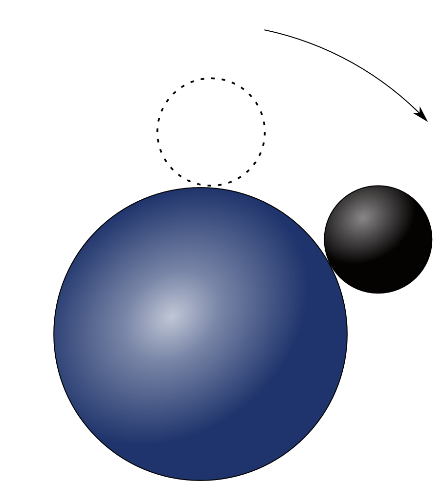
Puzzle: Roll a ball of unit radius on a fixed ball of radius , being careful not to let your ball slip or twist as you roll it. Suppose you roll along a great circle from the North Pole to the South Pole and back to the start at the North. How many turns did the ball make as it rolled?
Here’s a variant of this puzzle you can work out very concretely: for , roll one coin around another of the same kind, without slipping, and count the number of times the rolling coin turns.
Below the fold, I’ll give you the answer, and I’ll also tell you about something amazing that happens when , bringing in the exceptional Lie group and a funky 8-dimensional number system called the split octonions.
When Cartan and Killing classified the simple Lie groups, they found something unexpected. Besides the perfectly respectable infinite families, , and , there were five exceptions. In order of increasing dimension, these exceptional groups are prosaically called , , , and . While the first three kinds of groups are all symmetry groups of vector spaces equipped with some kind of bilinear form, the exceptions do not, at first glance, have a reason to exist. I like to imagine Cartan and Killing reacting like physicist I.I. Rabi to the discovery of the muon: “Who ordered that?” Since their discovery, finding simple models for the exceptional Lie groups has been an important program in mathematics. Here, I’ll tell you about one such model for , essentially due to Cartan: is almost the symmetry group of one ball rolling without slipping or twisting on another ball, provided the ratio of radii is 1:3 or 3:1.
When Jim Dolan and I started talking about this problem, we set out specifically to explain that funny ratio. We took our cue from Bor and Montgomery, who in their excellent paper G2 and the rolling distribution, write:
Open problem. Find a geometric or dynamical interpretation for the “3” of the 3:1 ratio.
Why only 1:3 or 3:1? You can see a hint of “threeness” in the Dynkin diagram for :

And that’s probably responsible for the 1:3 ratio, but by the end of the post, I’ll have shown you another explanation, far more geometric in nature. The key is going to be to relate the rolling ball picture to another description of , also due to Cartan: is the automorphism group of the ‘split octonions’, .
I’ll explain all of these ideas, so don’t worry if you’re unfamiliar with them. But first, an aside to those in the know: throughout this post, I’ll focus on the adjoint, split real form of , which is the only form for which all of these ideas make sense, though a lot of them continue to work for the complex form as well, as long as you replace the split octonions with their complexification. This is in keeping with a well-known theme in Lie theory: split real forms and complex forms behave in almost identical fashion.
The rolling ball
Now let’s get down to business, by working out a mathematical framework to describe a ball rolling on another ball, without slipping or twisting. To start off, I’ll let the fixed ball have radius , and the rolling ball have radius 1. Only later will we see what happens when we set .
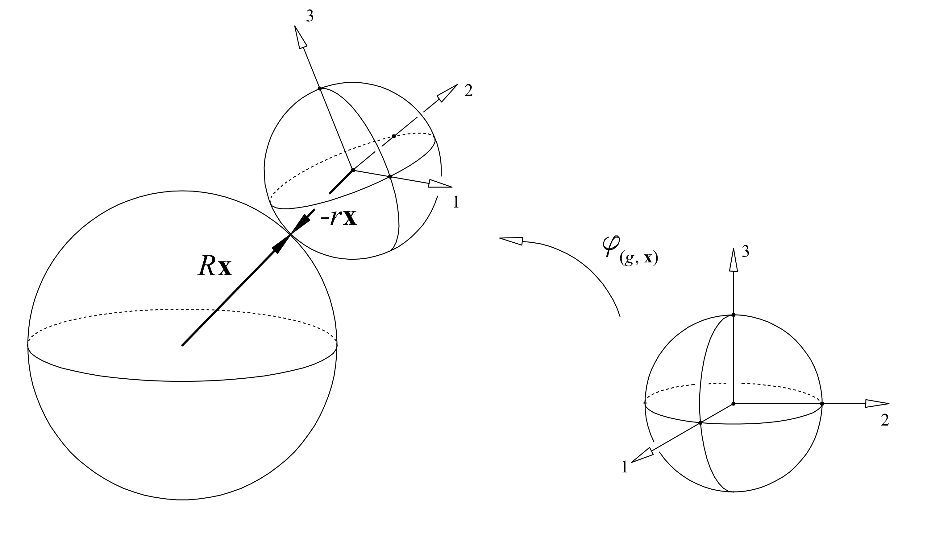
First, a configuration of this system corresponds to a point in , as follows: for , is the point of contact where the rolling ball touches the fixed ball, and tells us the present orientation of the rolling ball, rotating it from your favorite starting orientation. To show you what I mean, I can’t do better than a picture from the paper of Bor and Montgomery (though note that what I call they call , and they let their rolling ball have arbitrary radius ):
That’s how we describe configurations of the rolling ball system. What does it mean for the ball to roll without slipping or twisting? To describe that, we will turn to ‘incidence geometry’. This kind of geometry sounds very bare bones: in its simplest incarnation, an incidence geometry has points, lines, and an incidence relation (a point lies on a line, or is incident on the line). Yet this minimal structure will suffice to capture what we mean by rolling without slipping or twisting.
The rolling ball system defines an incidence geometry where:
- Points are configurations of the rolling ball—elements of .
- Lines are given by rolling without slipping or twisting along great circles.
A line, then, is some one-dimensional submanifold of . Which one-dimensional submanifolds are lines? Well, that’s the point of the puzzle at the start of this post. If you didn’t think about it before, go back and give it a shot now!
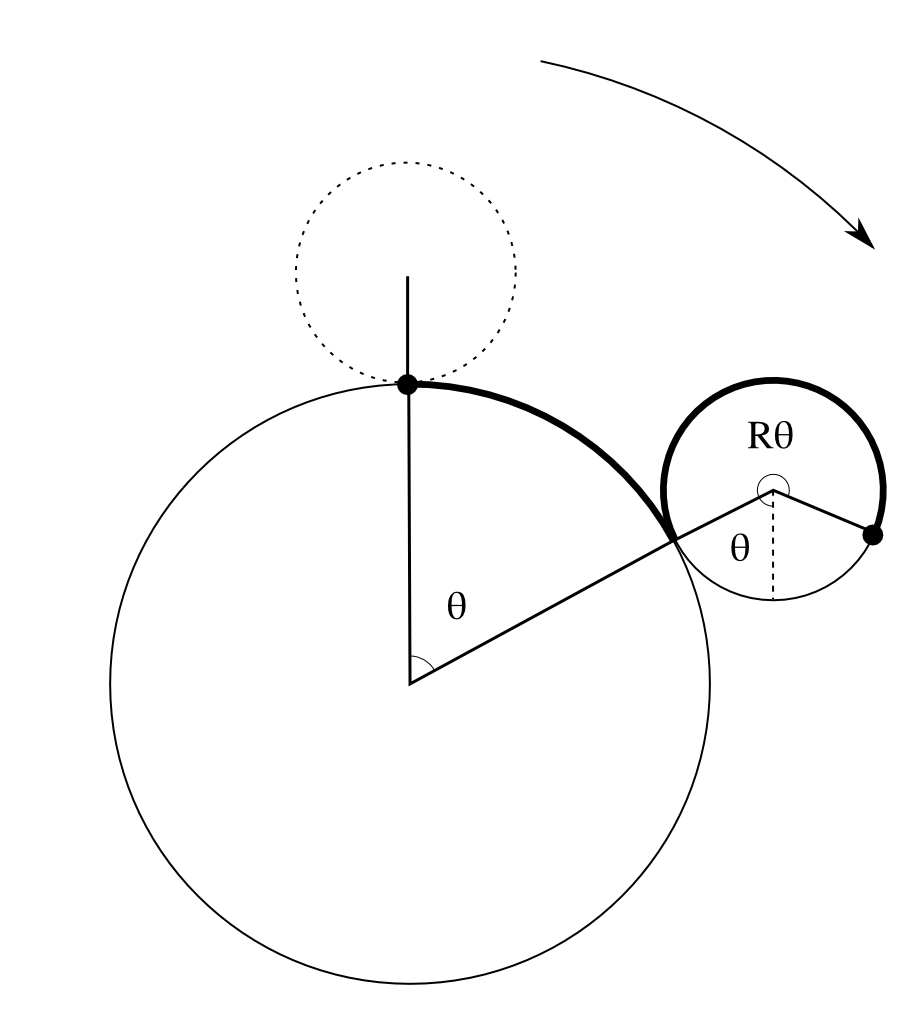
Here’s the answer: each time we roll a ball of unit radius around a ball of radius , the rolling ball turns times! And that’s how we roll. For instance, if begin rolling from the North Pole and sweep out a central angle as we do so, we rotate our ball by an angle about the axis going into the picture:
Now that we have a incidence geometry, we can talk about its symmetries. These symmetries are the diffeomorphisms that preserve the lines: Since the lines depend on , so does this group. Alas, this group is not , even when .
Remember, I said that was almost the symmetry group of the rolling ball, and we have run head first into that “almost”: as shown by Bor and Montgomery, does not act on . Instead, it acts on its double cover: And, if we stretch our imaginations a bit, we can think of this as a variant of the rolling ball system, which we call the ‘rolling spinor’.
The rolling spinor…
What’s a rolling spinor? It’s like a ball, but thanks to the “double” in the double cover , a rotation does not act like the identity. Instead, we need to rotate by degrees to get back where we started.
Spinors show up physically and mathematically. Famously, electrons are spinors, but a far more concrete example is given by the belt trick: put a twist in a belt, and you cannot undo the twist just by translating the ends around, but for twist, you can!
I can make more sense of this using quaternions. If I identify with the group of unit quaternions: and identify with the subspace of imaginary quaternions: than it’s easy for me to describe the covering map, . Each unit quaternion goes to the rotation of given by conjugation: The kernel of is . If I think of as giving a rotation by 0°, and as giving a rotation by 360°, then the idea that a 720° rotation is the identity becomes , which is indeed true. If this idea sounds funny, or you want an overview of quaternions, read this talk I gave at Fullerton College.
The rolling spinor system comes with an incidence geometry where:
- Points are elements of .
- Lines are preimages of lines in .
When , acts on as symmetries preserving lines. To understand this action, it helps to introduce yet another variant of the rolling ball system: the rolling spinor on a projective plane.
…on a projective plane
This system is double-covered by the rolling spinor: where the map identifies antipodal points of . We write for the equivalence class containing and . There is an incidence geometry where:
- Points are elements of .
- Lines are images of lines in .
Unlike the original rolling ball system, when , acts as symmetries of this incidence geometry. To see why, it’s time to introduce the split octonions.
Split octonions
The split octonions are an eight dimensional real composition algebra. There are two such algebras over the reals, the other being their more famous cousin, the octonions. We can define the split octonions as pairs of quaternions: with the following multiplication: Here, the barred quaternions and denote the conjugate, in , of and , obtained by flipping the sign of the imaginary part, just as we would do for a complex number. With this multiplication, one can check that the quadratic form: makes into a composition algebra, with the property:
Now we can define . And, as promised, this description of can be related to the rolling ball descriptions I have been sketching. But first, it helps to note that we don’t really need all of : since fixes , we really only need the subspace of imaginary split octonions. This is the subspace orthogonal to 1 with respect to . In terms of pairs of quaternions, this is the subspace where the first quaternion is purely imaginary while the second can be arbitrary: acts on the imaginary split octonions as well, and in fact it is the smallest irreducible representation of .
We’re close now. Because preserves , acts on the space of 1d null subspaces of : This space of null lines is almost the configuration space of the spinor rolling on the projective plane, . Choosing a representative of each line in , we can normalize its first component to have length 1, forcing the second component to also have unit length. Doing this, we see that: This ought to remind you of the spinor rolling on a projective plane, which has configuration space: In the first case, we mod out both components by their sign, and in the second, we just mod out the first. And in fact, these spaces are diffeomorphic: Note that this is not true for the ordinary rolling ball. We needed to think about a spinor rolling on a projective plane.
Under the diffeomorphism above, lines in incidence geometry become submanifolds of . If and only if , these submanifolds ‘straighten out’: they are given by projectivizing 2-dimensional null subspaces of the imaginary split octonions .
However, not all 2d null subspaces of yield lines in . When , the incidence geometry of coincides with the incidence geometry on with:
- Points are 1d null subspaces of .
- Lines are 2d null subspaces of on which the product also vanishes.
In fact, if we call a subspace of a null subalgebra if the product of any two elements vanishes, we can give a very snappy description of the incidence geometry on , thanks to the helpful fact that a 1d subspace of is null if and only if :
- Points are 1d null subalgebras of .
- Lines are 2d null subalgebras of .
Now we have what we wanted: the geometry of a spinor rolling on a projective plane, when , is the geometry of null subalgebras of the imaginary split octonions, . Hence, acts as symmetries of the spinor rolling on the projective plane!
Coda
We’ve seen how a spinor rolling on a projective plane three times as big acquires symmetry, but we still haven’t seen a completely satisfying explanation of that 1:3 ratio. It’s hiding somewhere in the proofs of the theorems I described above.
Yet there is an intuitive way to see the 1:3 ratio. Let’s think of our spinor as a ball that comes back to itself after turning twice, and let’s think of our projective plane as a ball with antipodal points identified. Rolling from a point on our fixed ball to its antipode, we’ve come back to where we’ve started in our projective plane. For what ratio of radii will the rolling spinor also be back where it started? That is, for what ratio of radii does the rolling ball turn an even number of times as it goes from a point to its antipode? At minimum, we need to turn twice. So:
- For what ratio of radii does the rolling ball turn twice as it goes from a point to its antipode? Or, put another way, for what ratio of radii does the rolling ball turn four times as it rolls once around the fixed ball?
By the solution to our puzzle, a ball of unit radius turns times as it rolls once around a fixed ball of radius . To turn four times, we need .
Re: G2 and the Rolling Ball
Huzzah!
Remember how we thought there might be some relation between the rolling ball and a pair of qubits, or something like that? I forget exactly how it worked. Do you remember?
Anyway, Cliff Harvey had an interesting post on G+ about entanglement for qubits, division algebras, and the Cayley–Dickson construction… even going up to the sedenions! I would like to figure out what’s going on here. The most intriguing paper is this: