Skip to the Main Content

Note:These pages make extensive use of the latest XHTML and CSS Standards. They ought to look great in any standards-compliant modern browser. Unfortunately, they will probably look horrible in older browsers, like Netscape 4.x and IE 4.x. Moreover, many posts use MathML, which is, currently only supported in Mozilla. My best suggestion (and you will thank me when surfing an ever-increasing number of sites on the web which have been crafted to use the new standards) is to upgrade to the latest version of your browser. If that's not possible, consider moving to the Standards-compliant and open-source Mozilla browser.

October 10, 2009

More Magnitude of Metric Spaces and Problems with Penguins

Posted by Simon Willerton

I have just about finished a paper on the magnitude of metric spaces, for which comments, corrections or questions are welcome.

This paper provides more motivation for the asymptotic conjecture in my paper with Tom Leinster described in a recent post by Tom.

As the title suggests, at the core of this paper are some back-of-the-envelope calculations and some big number crunching with Maple. The former leading to some conjectures which are supported by the latter.

I have two questions for patrons of the Café, the first of which does not require any familiarity with the paper.

  1. Is there a natural phenomenon which decreases exponentially with distance (as opposed to decreasing exponentially with time)?
  2. Is there a better term than ‘penguin valuation’ for the invariant valuation PP that is defined in the paper?

I will use motivating those two questions as an excuse to describe the contents of the paper.

To start with the first question, let me first remind you of the definition of a weighting of a finite metric space that was given in the paper with Tom (it didn’t appear in his original metric spaces post).

Suppose that XX is a finite metric space. A weighting on XX is an assignment of a weight w xw_x\in \mathbb{R} to each point in xXx\in X such that for each xXx'\in X the weight equation for xx' is satisfied: xXe d(x,x)w x=1.\sum_{x\in X} e^{-d(x,x')}w_x =1.

If a weighting for XX exists then |X||X|, the magnitude of XX is defined to be the sum of the weights:

|X| xw x.\left|X\right|\coloneqq\sum_x w_x.

This algebraic description comes by analogy with Tom’s corresponding definitions for finite categories, but it doesn’t come with any intuition, at least not for me. So I developed the following picture. Each point in XX is thought to be an organism which can regulate the amount of heat it generates (or absorbs). The amount of heat that the organism xx is generating is given by the weight w xw_x, where a negative weight indicates that heat is being absorbed, or, in other words, some kind of refrigeration or air-conditioning is happening at the point xx. The amount that the generated heat is felt falls off exponentially with distance from the organism. Each organism wishes to maintain a constant body temperature of one unit and they all regulate their heat to achieve that: this translates into precisely the weight equations being satisfied.

Now, I realise that there are many problems with that picture, however I do find it helpful and it does give me some kind of useful intuition — I’ll mention some related things below. But this does lead to the first question as to whether one can think of any genuine phenomena which decay exponentially with distance. A chemist friend mentioned possibly short-range repulsion of molecules, but I couldn’t really find anything on the internet about that.

Before getting to the second question, I should add that the original analogy that I had in mind was that the weight represented the ‘ego’ of an organism (or person or amoeba as I sometimes thought of them); so a positive weight represented extroversion and a negative weight represented introversion. The weight equation then represented the idea that the strength of someone’s personality drops off exponentially with distance and that each organism needed a certain level of ‘companionship’ so as not to go insane — so if they were very isolated they needed a strong extrovert personality to make up for it. However, it was pointed out to me that this perspective was rather artificial, unbelievable and idiosyncratic. Richard Thomas helped me come up with this, seemingly more acceptable, heat analogy.

Here’s an example of a weighting which demonstrates the analogy. In the picture below, we take the metric space to be a grid of points on a square in 2\mathbb{R}^2. The area of is proportional to the weight of the point at its centre, with a red disc meaning a positive weight and a blue disc meaning a negative weight.

Weighting on square grid

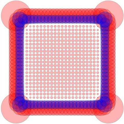
Tom pointed out to me that this is reminiscent of emperor penguins huddling on the Antarctic ice over the winter – you can see this in a clip of the BBC’s Life In The Freezer series. The penguins in the middle of the huddle are nice and cosy, being surrounded by other warm bodies, whereas the penguins on the edge of the huddle are more exposed and have to use up more energy generating heat. In the above picture of the weighting on the square grid, you see that the ‘penguins’ on the boundary have to generate so much heat to keep warm that the ones just inside from the boundary have to ‘switch on the air-conditioning’ (i.e., have negative weight as represented by the blue discs) in order not to get too hot.

What we are actually interested in are compact metric spaces rather than just finite ones. We can try to define the magnitude of a compact metric space XX by picking as sequence {X i} i=1 \{X_i\}_{i=1}^\infty of finite subsets of XX with X iXX_i\to X in the Hausdorff topology and defining the magnitude of XX to be the limit of the magnitude of these finite approximations to XX: so |X|lim i|X i|\left|X\right| \coloneqq \lim_i\left|X_i\right|. Whilst we don’t know that this works in general, it does seem to work for compact subsets of Euclidean spaces. The definition means that a good approximation to the magnitude of a compact set (if it exists) can be obtained by calculating the magnitude of a suitably dense finite subset.

Now suppose XX is the closure of an open subset of n\mathbb{R}^n, for instance a square in 2\mathbb{R}^2. Then if XX is ‘large’ you can do a heuristic argument to estimate the contribution to the magnitude of XX from the points in the ‘bulk’ of XX (or from the ‘cosy penguins’ if you will). Denoting the volume of the nn-dimensional ball by ω n\omega_n, the estimate of this bulk contribution is

Vol(X)n!ω n.\frac{\text{Vol}(X)}{n!\,\omega_n}.

I have no idea how to give a similar heuristic for what is happening at the boundary – in particular I can’t quantitatively explain the negative weights. However I can come up with a functional which seems to give the right answer in several cases. For this you need to recall the intrinsic volumes which I denote by μ n,μ n1,,μ 0\mu_n,\mu_{n-1},\dots,\mu_0, but which Tom denoted by || n,|| n1,,|| 0\left|\cdot \right|_n, \left|\cdot \right|_{n-1}, \dots, \left|\cdot \right|_0 in his metric spaces post. These are defined on certain compact subsets of n\mathbb{R}^n: I’m not sure of the exact domain of definiton, but they are certainly defined on finite unions of convex sets and and smooth submanifolds. They have various properties, but the pertinent ones here are μ n(X)=Vol(X)\mu_n(X)=\text{Vol}(X) and μ i(X)\mu_i(X) for i<ni\lt n can be localized to the boundary. For instance, μ n1(X)\mu_{n-1}(X) is half the “surface area” of XX, or half the (n1)(n-1)-volume of the boundary, if you prefer; and μ 0(X)\mu_0(X) is the Euler characteristic of XX.

Motivated by a wild assumption of some kind of naturality, define the functional

P(X) i=0 nμ i(X)i!ω i.P(X)\coloneqq\sum_{i=0}^{n} \frac{\mu_i(X)}{i!\,\omega_i}.

By the properties of the intrinsic volumes mentioned above, P(X)P(X) is of the form

estimate of contribution from the bulk+terms from the boundary.\text{estimate of contribution from the bulk}+\text{terms from the boundary}.

When n=2n=2 we have

P(X)=12πArea(X)+12Perimeter(X)+EulerChar(X).P(X)= \tfrac{1}{2\pi}Area(X) + \tfrac{1}{2}Perimeter(X) + EulerChar(X).

We’re just about ready for the second question now, but let’s conclude the mathematics first. The functional P(X)P(X) seemed to be a bit of a guess at some estimate of the magnitude |X|\left| X\right| when XX is a ‘large’ space. The amazing thing, and one of the key points of the paper, is that for squares, discs and cubes, i.e., the convex spaces that I did calculations for, these two functionals seem to agree to a large extent. So one is led to conjecture that

|K|=P(K)forKconvex.\left|K\right|=P(K)\quad {for K convex}.

One the other hand, for annuli and tori these two functionals just seem to agree asymptotically, meaning that if we denote by tXtX the metric space with distance scaled up by a factor tt then

|tX|P(tX)0ast.\left|tX\right|-P(tX)\to 0\quad as\quad t\to \infty.

The paper includes some nice graphs of this behaviour. However, it is important to say here [which I didn’t do before David Speyer reminded me] that I don’t know what sort of spaces to expect this asymptotic behaviour for (other than the closure of open sets of Euclidean space ). In particular, David Speyer pointed out in an earlier post the case of the bent line in which two straight line segments are stuck together at an angle: numerical calculations for the magnitude seem to show a small, constant discrepancy with the penguin valuation. I have also done some asymptotic analysis with the 33-sphere which seems to show that the lower order terms are not right in that case – however I’m not so confident in the calculations at the moment.

Now to get to the question. What can I call PP? I tried to think of a name for it for a long time. In the end I plumped for the term ‘penguin valuation’ for the following reasons.

  1. I couldn’t think of anything else.
  2. In the paper with Tom the symbol PP had already been used for it.
  3. [Erm, a bit weak this one, and thought up afterwards.] It does kind of create an image in the mind of contribution from the cosy penguins and from the penguins on the boundary.

However, some might find the term overly whimsical. Does anyone have any better ideas?

I’ll finish with a trivia question for you.

  • What’s the connection between the Leicester mathematics department and the BBC penguin video?
Posted at October 10, 2009 11:01 PM UTC

TrackBack URL for this Entry:   https://golem.ph.utexas.edu/cgi-bin/MT-3.0/dxy-tb.fcgi/2080

131 Comments & 3 Trackbacks

Re: More Magnitude of Metric Spaces and Problems with Penguins

I haven’t even looked at the paper yet (I will!) and haven’t even finished reading your post, but thought I would go ahead and respond to this:

Is there a natural phenomenon which decreases exponentially with distance (as opposed to decreasing exponentially with time)?

A plane wave (in Fourier space) can be expressed as

exp[i(kx+ωt)]exp\left[i\left(k\cdot x + \omega t\right)\right]

When the material is lossy, the wave vector kk decomposes into a real and imaginary parts k=k+ikk = k' + i k'' so we’ve got:

exp(kx)exp[i(kx+ωt)]exp(-k''\cdot x) exp\left[i\left(k'\cdot x + \omega t\right)\right]

which is a plane wave whose amplitude decreases exponentially with distance from the source.

That may or may not help. Back to the post! :)

Posted by: Eric Forgy on October 12, 2009 12:18 AM | Permalink | Reply to this

Re: More Magnitude of Metric Spaces and Problems with Penguins

Ok! I’ve now read the post, but not the paper yet (I will!).

I like the heat analogy. Is it possible that what you denote d(x,x)d(x,x') should rather be associated with the square of a distance? That would aid the analogy.

I really like the example and the comparison to penguins :)

The “lossy wave” example I gave of a physical phenomenon with exponential decrease with distance will not help because the various sources will superpose with phase difference, so there will be interference patterns. Not to mention for point sources there would be a 1/r1/r dependence in addition to the e re^{-r} dependence.

What you want is a static phenomenon (with no wave interference). Heat is interesting, but you’d need distance squared.

Next is to read the paper! :)

Posted by: Eric Forgy on October 12, 2009 2:50 AM | Permalink | Reply to this

Re: More Magnitude of Metric Spaces and Problems with Penguins

Eric said

Heat is interesting, but you’d need distance squared.

I guess that would be the case for subsets of 3\mathbb{R}^3. For n\mathbb{R}^n I would expect heat in a vacuum at a distance rr from a point source to be felt like 1/r n11/r^{n-1}. We want an effect that is independent of the ambient dimension, which seems a bit odd to me.

Posted by: Simon Willerton on October 12, 2009 2:52 PM | Permalink | Reply to this

Re: More Magnitude of Metric Spaces and Problems with Penguins

Hi Simon,

Here is the expression for the heat kernel in dd-dimensions:

K(t,x,y)=1(4πt) d/2exp(|xy| 24t).K(t,x,y) = \frac{1}{(4\pi t)^{d/2}} \exp\left(-\frac{|x-y|^2}{4t}\right).

This varies exponentially with the square of distance in any dimension.

It still doesn’t necessary help you though.

Posted by: Eric Forgy on October 12, 2009 3:38 PM | Permalink | Reply to this

Re: More Magnitude of Metric Spaces and Problems with Penguins

Simon wrote:

For n\mathbb{R}^n I would expect heat in a vacuum at a distance rr from a point source to be felt like 1/r n11/r^{n-1}.

You’re talking about the radiative power per ‘area’ at a distance rr from a point source of radiation. (‘Area’ in quotes because that’s the right word only for n=3n = 3.)

Eric is talking about the temperature at time tt at a distance rr away from a given point, where at time zero the temperature distribution was a delta function located at that point. In other words, he’s talking about the fundamental solution of the heat equation, also known as the ‘heat kernel’.

I know of nothing in physics that decays in a way proportional to e constantre^{-constant r}, except when space is 1d. As others have hinted, a force that’s carried by a particle of mass mm decays in a way proportional to e mr/r n1e^{- m r}/ r^{n-1}, where nn is the dimension of space.

This was Yukawa’s great idea, the one that that led him to predict the existence of the pion. It’s also what’s lurking behind your chemist friend’s remark, insofar as I understand it. I could explain more about his remark if you like, but first the bad news: the decay of these forces is only exactly proportional to an exponential when n=1n = 1.

Posted by: John Baez on October 12, 2009 10:00 PM | Permalink | Reply to this

Re: More Magnitude of Metric Spaces and Problems with Penguins

John said:

I could explain more about his remark if you like.

Yes please. Although if you meant the remark of my chemist friend, then it would be her remark.

Posted by: Simon Willerton on October 14, 2009 2:46 AM | Permalink | Reply to this

Re: More Magnitude of Metric Spaces and Problems with Penguins

Thanks John. That’s the kind of explanation I was after.

Posted by: Simon Willerton on October 14, 2009 8:45 AM | Permalink | Reply to this

Re: More Magnitude of Metric Spaces and Problems with Penguins

Okay. In 3d space, if you have a stationary electrically charged particle in the vacuum, it pushes on other such particles with a force proportional to 1/r 21/r^2. This is called Coulomb’s law.

But now suppose you have a stationary charged particle in water. And suppose, just for the sake of definiteness, that this particle is negatively charged — say, an electron.

By what I said before, your electron will push on all the other negatively charged parts of the surrounding water molecules, and pull on all the positively charged parts. But since these forces counteract, they won’t accelerate the water molecules. Instead, they’ll actually stretch the water molecules, so the positively charged parts are further away, and the negatively charged parts are closer. We say the surrounding water molecules are ‘polarized’.

But this in turn will create a counteracting electric field, since it means that if you draw any sphere around your electron, there will be a bit more positively charged other stuff in that sphere than negatively charged other stuff! The bigger the sphere is, the more this effect occurs — though there is a limit to how much it occurs.

We say that the further you go from your electron, the more its electric charge is screened, or hidden, behind the effect of the polarization. And, to a reasonable approximation, the result is to change the 1/r 21/r^2 force law to a modified law like this:

e k 0rr 2 \frac{e^{-k_0 r }}{r^2}

for some constant k 0k_0, which describes how strong the screening is. So, we get something like exponential decay… but it’s really an exponential times 1/r 21/r^2. Materials in which this effect occurs are called dielectrics.

Note this exponential-times-1/r 21/r^2 force law is just like the Yukawa force law for the force carried by a massive particle. That’s because the same differential equation is involved.

If we repeated the analysis in nn-dimensional space, we’d get a force proportional to

e k 0rr n1 \frac{e^{-k_0 r }}{r^{n-1}}

Only when n=1n = 1 do we get precisely exponential decay.

And indeed, this agrees with what Eric was telling you about wave transmission through a lossy medium. He was talking about waves in nn dimensions… but only for plane waves does the problem reduce to an effectively 11-dimensional problem, giving us exponential decay.

Indeed, I don’t think you’ll find any physical phenomena that decay (almost) exactly exponentially with distance, except in 1d space. The problem is that in higher dimensions, partial differential equations that are invariant under rotations and translations just don’t have solutions like exp(k 0r)exp(-k_0 r).

Posted by: John Baez on October 14, 2009 3:36 AM | Permalink | Reply to this

Re: More Magnitude of Metric Spaces and Problems with Penguins

Note that in liquid water, the molecules can not only stretch but also rotate, moving their positive parts closer to the electron and their negative parts further away, and this is the stronger effect.

Posted by: Tim Silverman on October 14, 2009 12:55 PM | Permalink | Reply to this

Re: More Magnitude of Metric Spaces and Problems with Penguins

You know, the more I look at that picture, the more I’m reminded of the Strong Force, which I keep hearing decays exponentially, and is particularly unhelpful to “peripheral” nucleons in larger and larger nuclei … although I suppose “peripheral” would be the semi-classical word for it…

Anyways, I’m not being any more coherent than my usual self, so by all means, keep “penguin”. Laymen might wonder has it anything to do with the cat map.

Posted by: some guy on the street on October 12, 2009 1:42 AM | Permalink | Reply to this

Re: More Magnitude of Metric Spaces and Problems with Penguins

One thing I don’t understand is what the mechanism for an exponentially decaying effect would be. I can see how we get the inverse square law in three-dimensions by imagining how at a distance rr the effect is smeared out over a sphere of surface area 4πr 24\pi r^2 but I can’t see how anything like that would work for exponential decay. How is the Strong Force supposed to be mediated, for instance?

Posted by: Simon Willerton on October 12, 2009 3:16 PM | Permalink | Reply to this

Re: More Magnitude of Metric Spaces and Problems with Penguins

On the level of nucleons, the strong force can be described as an effective interaction mediated through pion exchange. Since pions are massive, the force is described by the Yukawa potential having the form e mrr\frac{e^{-mr}}{r}. The exponential decay is due to the exponential decay of a massive particle’s propagator.

(I’m anything but an expert on this, so please take my words with a grain of salt.)

Posted by: Tobias Fritz on October 12, 2009 3:54 PM | Permalink | Reply to this

Re: More Magnitude of Metric Spaces and Problems with Penguins

So every force is inverse square at short range and exponential decay at long range. By dimensionalysis, the boundary between short and long range should be the Compton wavelength of the mediating particle; if the mediator's mass is zero, then every range is short. One way (probably not the tightest way) to get an upper bound on the mass of a photon (which we think is zero but which conceivably might be positive) is to see how far out you can measure that electromagnetism satisfies an inverse square law.

Posted by: Toby Bartels on October 12, 2009 9:00 PM | Permalink | Reply to this

Re: More Magnitude of Metric Spaces and Problems with Penguins

I think I already mentioned this to you in an e-mail, but that’s no reason not to say it again: I understand weightings as describing a collection of particles which repel each other with potential energy e d(x,y)e^{-d(x,y)}.

Let’s start by thinking about a finite metric space with nn points. Let’s suppose we have a total charge of 11 available, and we want to distribute it among the nn points, putting p ip_i on point ii, while minimizing the energy p ip je d(i,j)\sum p_i p_j e^{- d(i,j)}. A quick computation (for example, by Lagrange multipliers) shows that the critical points of this functional are given by weightings. The fact that weightings can be negative is a little weird from this analogy, but I can live with it.

One very interesting question is for which metric spaces MM the inner product p ip je d(i,j)\sum p_i p_j e^{-d(i,j)} is positive definite on M\mathbb{R}^M. For such a metric space, if we choose any function ww in M\mathbb{R}^M with w(i)=1\sum w(i)=1 then 1/p ip je d(i,j)1/\sum p_i p_j e^{-d(i,j)} is a lower bound for the magnitude of the metric space. This means it is fantastically easy to give rigorous lower bounds in these cases. In particular, if MM has this property than every subspace of MM does, and it is easy to see that the magnitude of NN is less than MM for every NMN \subseteq M. I also think that it should be easy to clean up all issues related to approximation by finite metric spaces in this setting.

In fact, I’ll throw out a wild conjecture: For x 1x_1, … x nx_n any finite subset of Euclidean space, the matrix e d(x i,x j)e^{-d(x_i, x_j)} is positive definite.

Posted by: David Speyer on October 12, 2009 5:43 AM | Permalink | Reply to this

Re: More Magnitude of Metric Spaces and Problems with Penguins

David wrote:

One very interesting question is for which metric spaces MM the inner product p ip je d(i,j)\sum p_i p_j e^{-d(i, j)} is positive definite

I agree: this is an important property, partly because it makes the passage to compact spaces much smoother.

I call a finite metric space positive definite if it has this property — that is, its similarity matrix is positive definite. As usual, the similarity matrix ZZ of a metric space {a 1,,a n}\{a_1, \ldots, a_n\} is the n×nn\times n matrix defined by Z ij=e d(a i,a j)Z_{i j} = e^{-d(a_i, a_j)}.

Here are some classes of (finite) positive definite metric space:

  1. ultrametric spaces, i.e. those satisfying the stronger version d(a,c)max{d(a,b),d(b,c)} d(a, c) \leq max \{ d(a, b), d(b, c) \} of the triangle inequality
  2. scattered metric spaces, i.e. nn-point spaces satisfying d(a,b) > 1/(n1)d(a, b) &nbsp;&gt;&nbsp; 1/(n - 1) for all points aba \neq b
  3. metric spaces with 3\leq 3 points
  4. subspaces of m\mathbb{R}^{\otimes m}, for any mm. Here m\mathbb{R}^{\otimes m} is m\mathbb{R}^m with the d 1d_1 or taxicab metric: d(a,b)= i|a ib i|d(a, b) = \sum_i |a_i - b_i|. (It’s called \otimes because it’s the tensor product of enriched categories.)

The proofs that the first three classes of space are positive definite are in my maximum entropy paper: Example 4.5, Example 4.6 and Lemma 2.20, respectively. The last class (subsets of m\mathbb{R}^{\otimes m}) isn’t in that paper; I’ll sketch a proof in a separate comment.

You might be interested, David, in some of the results on positive definite spaces on p.12-14 of the paper. In particular, there’s the following result (Lemma 2.18): the cardinality of a positive definite space with similarity matrix ZZ is sup x1x tZx \sup_{\mathbf{x}} \frac{1}{\mathbf{x}^t Z \mathbf{x}} where the supremum is over all x n\mathbf{x} \in \mathbb{R}^n such that x i=1\sum x_i = 1. You mentioned a part of this result (though I suspect you know the whole thing). Incidentally, it’s really ZZ, not the metric space, that’s the central player here; we don’t need the triangle inequality at all.

As for your conjecture (slightly rephrased)…

any finite subset of Euclidean space is positive definite

…I don’t know. I’ve tried to prove it and I’ve tried to disprove it, to no avail. If you can do it, great!

Posted by: Tom Leinster on October 12, 2009 1:27 PM | Permalink | Reply to this

Re: More Magnitude of Metric Spaces and Problems with Penguins

Machine learning people are hot on the idea of using the kernel trick to map a feature space and its similarity metric to a higher-(possibly infinite) dimensional space where linear classifier algorithms can be applied.

They need kernels with (semi-) positive definite Gram matrices to measure the similarity between inputs. A very common kernel is the Gaussian, which takes the similarity for points in n\mathbb{R}^n to be

k(x,y)=exp(xy 2). k(x, y) = exp(-\Vert x - y \Vert^2).

I think I’m right in saying that for nn distinct points the n×nn \times n matrix k(x i,x j)k(x_i, x_j) is positive definite.

But I never heard of them using exp(xy)exp(-\Vert x - y \Vert).

Posted by: David Corfield on October 12, 2009 3:02 PM | Permalink | Reply to this

Re: More Magnitude of Metric Spaces and Problems with Penguins

The Gaussian distribution (which is closely related to the heat kernel) is a special case of a stable distribution with α=2\alpha = 2 (α=2\alpha = 2 leads the exponential of distance squared dependence). It’s characteristic function is

exp(it|ct| 2).\exp\left(it - |ct|^2\right).

Setting β=0\beta = 0, the more general stable characteristic function is

exp(it|ct| α).\exp\left(it - |ct|^\alpha\right).

I might be sending you on a wild goose chase, but it might interesting to look the case α=1\alpha = 1. I would have hoped this gave rise to a probability density (and hence kernel for some PDE via Feynman-Kac) of the form

exp(|xy|)\exp\left(-|x-y|\right)

but, alas, that is not the case. Setting α=1\alpha = 1 and β=0\beta = 0 leads to the Cauchy distribution for which I’m not very familiar.

Nevertheless, it may help in your pursuit to consider that kernels relate to PDEs and PDEs relate to physical phenomenon. So maybe we can try to see what PDE the kernel exp(|xy|)\exp(-|x-y|) corresponds to. It is not obvious to me because I have not had my coffee yet :)

Posted by: Eric Forgy on October 12, 2009 4:02 PM | Permalink | Reply to this

Re: More Magnitude of Metric Spaces and Problems with Penguins

There’s also some connection to the logistic distribution. Give or take some constants, the probability density function of the logistic distribution is sech 2sech^2.

The connection is this. Let AA be a compact subset of \mathbb{R}. For xx \in \mathbb{R}, write d(x,A)=inf aAd(x,a)d(x, A) = inf_{a \in A} d(x, a). Then |A|= sech 2d(x,A) dx. |A| = \int_{-\infty}^\infty sech^2 d(x, A) &nbsp; d x. (At least, that’s correct modulo some factors of 22, which I’m not going to attempt to get right.)

Posted by: Tom Leinster on October 12, 2009 5:35 PM | Permalink | Reply to this

Re: More Magnitude of Metric Spaces and Problems with Penguins

It looks as though

k(x,y)=exp(xy/θ) k(x, y) = exp(- \Vert x - y \Vert/\theta)

is a kernel. It is called the ‘exponential kernel’, e.g., here. But note that elsewhere the term is used for another kernel.

This kernel is positive definite in d\mathbb{R}^d, which entails Tom’s rephrasing of David S.’s conjecture.

Posted by: David Corfield on October 12, 2009 5:32 PM | Permalink | Reply to this

Re: More Magnitude of Metric Spaces and Problems with Penguins

Wait: I’m struggling with the terminology here. Are you saying that, according to this paper, every finite subspace of n\mathbb{R}^n (with the Euclidean metric) is positive definite?

(This isn’t the greatest of my problems, but something that bothers me about the paper that you link to is the definition of positive definite: his equation (1). That looks more like the definition of positive semidefinite to me. E.g. according to him, the constant function K=0K = 0 is positive definite.)

Posted by: Tom Leinster on October 12, 2009 5:43 PM | Permalink | Reply to this

Re: More Magnitude of Metric Spaces and Problems with Penguins

Hmm, all that Mercer’s theorem business is about positive semidefinite (or non-negative definite) kernels, so you have a point.

On the other hand, I know that in the case of the Gaussian (squared-exponential) kernel that the matrix is positive definite so long as the points are distinct. It’s quite plausible that this still works for the exponential case.

Where can someone find a friendly functional analyst around here?

Posted by: David Corfield on October 12, 2009 6:00 PM | Permalink | Reply to this

Re: More Magnitude of Metric Spaces and Problems with Penguins

(Don’t know about friendly, but …)

I’m afraid I haven’t found time to read through Simon and Tom’s work, so forgive me if the following remarks are facile and have already been considered. But the conjecture “every subset of R nR^n is positive (semi-)definite” seems to be the same as asking if the function R nRR^n \to R, xe xx \mapsto e^{-\Vert x\Vert}, is positive semi-definite in the usual sense.

Do the results usually referred to as “theorems of Schoenberg” help here? See pages 2—3 of

arxiv.org/abs/math/0404401

Also, I think people have studied negative-definite kernels on discrete hyperbolic groups, but I’d have to go and trawl through my old bookmarks to check.

Posted by: Yemon Choi on October 12, 2009 9:51 PM | Permalink | Reply to this

Re: More Magnitude of Metric Spaces and Problems with Penguins

The literature is terrible. No terms seem to be used with a fixed meaning. Just as one gets used to

k(x,y)=exp(xy) k(x, y) = exp(-\Vert x - y\Vert)

as the ‘exponential kernel’, it gets called the Laplace kernel, and ‘exponential kernel’ is used for something else (page 13, table 2.1).

Ah, this is relevant. We read

Theorem 10 (Positive Definite Kernel is Universal) A kernel is universal, if for arbitrary sets of distinct points it induces strictly positive definite kernel matrices.

And Theorem 8, a kernel is universal if and only if its Fourier coefficients are strictly positive. But the Fourier coefficients for the kernel

k(x,y)=exp(xy)/θ k(x, y) = exp(-\Vert x - y\Vert)/ \theta

are page 5 of this:

f(ω)=1πθ+πθω 2, f(\omega) = \frac{1}{\frac{\pi}{\theta} + \pi \theta \omega^2},

i.e., positive.

So the Laplace kernel is universal, but wait Theorem 10 didn’t say ‘if and only if’.

Hmm, a little confused.

Posted by: David Corfield on October 12, 2009 10:18 PM | Permalink | Reply to this

Re: More Magnitude of Metric Spaces and Problems with Penguins

Thanks, Yemon. I was hoping you’d pop your head up.

I spent last night reading this paper of Schoenberg:

I.J. Schoenberg, Metric spaces and positive definite functions, Transactions of the American Mathematical Society 44 (1938), 522-536.

You’re right: in the terminology that Schoenberg uses, the question is whether the function m,    xe ||x|| \mathbb{R}^m \to \mathbb{R}, &nbsp;&nbsp;&nbsp;&nbsp; \mathbf{x} \mapsto e^{-||\mathbf{x}||} is positive definite, for every nn.

Actually, we want to know a bit more. Schoenberg uses ‘positive definite’ where I’d want to use ‘positive semidefinite’; he asks only that something is 0\geq 0, placing no restrictions on when equality is attained. I don’t know what those who use Schoenberg’s terminology would call what I’d call ‘positive definite’ — ‘strictly positive definite’, perhaps? (David C’s comment suggests this.) Maybe you know?

In any case, we want to know whether e ||x||e^{-||\mathbf{x}||} is positive definite in the strict sense.

I don’t have a proof of this. But I think I can use Schoenberg’s results to prove that e ||x|| pe^{-||\mathbf{x}||_p} is positive semidefinite for all p[1,2]p \in [1, 2]. In other words, I think I can prove that if AA is a finite metric space that embeds in ( m,d p)(\mathbb{R}^m, d_p) for some mm \in \mathbb{N} and p[1,2]p \in [1, 2], then the similarity matrix (e d(a,b)) a,b(e^{-d(a, b)})_{a, b} of AA is positive-semidefinite. Here d pd_p is the pp-metric on m\mathbb{R}^m, given as usual by d p(x,y)=( i=1 m|x iy i| p) 1/p. d_p(\mathbf{x}, \mathbf{y}) = \left( \sum_{i = 1}^m |x_i - y_i|^p \right)^{1/p}. I’ll give the proof in a separate comment.

From Schoenberg’s other results I suspect that this fails for p > 2p &nbsp;&gt;&nbsp; 2. It certainly fails for p=p = \infty. Indeed, Schoenberg shows (p.535) that every finite metric space embeds in ( m,d )(\mathbb{R}^m, d_\infty) for some mm, and there are finite metric spaces that are not positive-semidefinite.

(Incidentally, Schoenberg says that this result is essentially due to Fréchet, citing a 1910 paper of his. I believe it was Fréchet who formulated the definition of metric space. It’s interesting that this result came so soon afterwards — or maybe even before.)

Posted by: Tom Leinster on October 13, 2009 4:53 PM | Permalink | Reply to this

Re: More Magnitude of Metric Spaces and Problems with Penguins

Oops: I missed this comment of David C, where he tells us that those who use ‘positive definite’ for the weaker condition use ‘strictly positive definite’ for the stronger one.

Posted by: Tom Leinster on October 13, 2009 5:10 PM | Permalink | Reply to this

Re: More Magnitude of Metric Spaces and Problems with Penguins

Hot off the press from a friend from Tübingen, we learn that

the Laplace kernel is indeed strictly positive definite. Interestingly, strictly positive definite kernels allow one to uniquely embed probability distributions (and not just individual points) in a reproducing kernel Hilbert space.

He sends me an unpublished paper with more on this, which I’ll report on soon.

Posted by: David Corfield on October 13, 2009 7:17 PM | Permalink | Reply to this

Re: More Magnitude of Metric Spaces and Problems with Penguins

Great! So we have a proof — well, a proof by authority, at least.

Posted by: Tom Leinster on October 13, 2009 7:38 PM | Permalink | Reply to this

Re: More Magnitude of Metric Spaces and Problems with Penguins

I promised to prove that for all mm \in \mathbb{N} and p[1,2]p \in [1, 2], the function m,    xe ||x|| p \mathbb{R}^m \to \mathbb{R}, &nbsp;&nbsp;&nbsp;&nbsp; \mathbf{x} \mapsto e^{-||\mathbf{x}||_p} is positive semidefinite. This is another way of saying that for a finite subset AA of m\mathbb{R}^m, the similarity matrix (e ||ab|| p) a,bA(e^{-||a - b||_p})_{a, b \in A} is positive semidefinite. Or to put it another way, any finite metric space that embeds in ( m,d p)(\mathbb{R}^m, d_p) for some mm and p[1,2]p \in [1, 2] is positive semidefinite.

I’ll use results from the paper of Schoenberg cited previously. Schoenberg uses ‘positive definite’ for what I’m calling ‘positive semidefinite’. Some facts:

  1. The product of positive semidefinite functions on m\mathbb{R}^m is again positive semidefinite (p.524, Property II).
  2. For p(0,2]p \in (0, 2], the function xe |x| px \mapsto e^{-|x|^p} on \mathbb{R} is positive semidefinite (p.532, Cor 3).
  3. Let ϕ: m\phi: \mathbb{R}^m \to \mathbb{R} be a homogeneous function and γ(0,1]\gamma \in (0, 1]. Suppose that e ϕe^{-\phi} is positive semidefinite. Then e ϕ γe^{-\phi^\gamma} is positive semidefinite (p.528, Cor 2).

    (‘Homogeneous’ means that there is some constant α\alpha such that ϕ(tx)t αϕ(x)\phi(t\mathbf{x}) \equiv t^\alpha \phi(\mathbf{x}), and e ϕ γe^{-\phi^\gamma} is the function xe ϕ(x) γ\mathbf{x} \mapsto e^{-\phi(\mathbf{x})^\gamma} on m\mathbb{R}^m.)

Let mm \in \mathbb{N} and p[1,2]p \in [1, 2]. Fact 2 easily implies that for each i{1,,m}i \in \{1, \ldots, m\}, the function xe |x i| p \mathbf{x} \mapsto e^{-|x_i|^p} on m\mathbb{R}^m is positive semidefinite. Fact 1 then implies that the function xe (|x 1| p++|x m| p) \mathbf{x} \mapsto e^{-(|x_1|^p + \cdots + |x_m|^p)} on m\mathbb{R}^m is positive semidefinite. Also, the function x|x 1| p++|x m| p \mathbf{x} \mapsto |x_1|^p + \cdots + |x_m|^p on m\mathbb{R}^m is homogeneous (of degree pp), and 1/p(0,1]1/p \in (0, 1]. So by Fact 3, the function xe (|x 1| p++|x m| p) 1/p \mathbf{x} \mapsto e^{-(|x_1|^p + \cdots + |x_m|^p)^{1/p}} is positive semidefinite, as required.

I’m optimistic that this can be improved to ‘positive definite’.

Posted by: Tom Leinster on October 13, 2009 5:54 PM | Permalink | Reply to this

Re: More Magnitude of Metric Spaces and Problems with Penguins

Apparently

Sun, X., Conditionally positive definite functions and their application to multivariate interpolation, J. Approx. Theory 74 No. 2, (1993), 159-180.

deals with strictly positive definite radial functions in d\mathbb{R}^d, but I don’t have access now.

Posted by: David Corfield on October 12, 2009 6:27 PM | Permalink | Reply to this

Re: More Magnitude of Metric Spaces and Problems with Penguins

Here on p. 3 it is claimed that

C. A. Micchelli, “Interpolation of scattered data: Distance matrices and conditionally positive definite functions,” Constructive Approximation, vol. 2, pp. 11–22, 1986

shows that the Gram matrix for a radial basis function kernel is positive definite and of full rank for distinct points.

Posted by: David Corfield on October 12, 2009 6:46 PM | Permalink | Reply to this

Re: More Magnitude of Metric Spaces and Problems with Penguins

Hmm, thanks. Unfortunately I don’t know what the following terms mean:

  • kernel
  • Gram basis
  • radial
  • basis function

…and very much else besides. I’m not asking you to explain what they mean. What I’d really like is if you’d indulge me for a moment and just tell me the answer: is it the case that what you’ve discovered in the literature implies that every finite subspace of m\mathbb{R}^m is positive definite?

I know you’ve only just found this stuff and I’m not asking for a guarantee — I’m just asking whether that’s the impression you have at the moment.

Thanks!

Posted by: Tom Leinster on October 12, 2009 7:13 PM | Permalink | Reply to this

Re: More Magnitude of Metric Spaces and Problems with Penguins

Well I can tell you what a kernel is. I ought to figure out how to say what it is in the language of enriched profunctors, but it’s been a long day so I won’t.

If XX and YY are spaces then a kernel is a function on X×YX\times Y which gives rise to a function from functions on XX to functions on YY via integral transform. So if k:X×Yk:X\times Y \to \mathbb{R} is a function and C(X)C(X) denotes the functions on XX then the corresponding transform T k:C(X)C(Y)T_k: C(X)\to C(Y) is given by

(T k(f))(y) Xk(x,y)f(x)dx(T_k(f))(y)\coloneqq \int_X k(x,y)f(x) dx

If XX and YY are not compact then to make this transform well-defined you need kk or ff to decay appropriately quickly. To say this properly you need to say carefully what kind of functions you are allowing. But I’m being vague.

[This is essentially the same idea as an AA,BB-bimodule giving rise to a functor from AA-modules to BB-modules.]

Really it’s like a continuous version of a matrix, and can be thought of as a linear map from functions to functions.

Posted by: Simon Willerton on October 12, 2009 9:15 PM | Permalink | Reply to this

Re: More Magnitude of Metric Spaces and Problems with Penguins

Yes, all this kernel business relates to John’s groupoidification program.

I wrote about kernels in learning theory before: I, II, III.

As for the key question that Tom wants to know, I’ll need to ask some old colleagues. It’s very easy to trip up here with people using the same terminology differently.

The one thing I do know is that if you asked me the same question for the matrix with (i,j)(i, j) entry equal to e d(x i,x j) 2e^{-d(x_i, x_j)^2}, then the answer would have been ‘yes’ – distinct points give us a strictly positive definite matrix.

Posted by: David Corfield on October 12, 2009 9:35 PM | Permalink | Reply to this

Re: More Magnitude of Metric Spaces and Problems with Penguins

Thanks, David.

Posted by: Tom Leinster on October 13, 2009 3:34 PM | Permalink | Reply to this

Re: More Magnitude of Metric Spaces and Problems with Penguins

When they say “radial basis function”, I don’t get the impression they mean “any radial basis function”. It looks like they have a specific form in mind, i.e. Equation (1), and exp(d)\exp(-d) is not a radial basis function (using their terminology).

Posted by: Eric Forgy on October 12, 2009 7:26 PM | Permalink | Reply to this

Survival of the Penguins

It is called the ‘exponential kernel’

Right right. This dawned on me after I had my coffee.

The physical interpretation is that “something” (a penguin?) has a constant probability of surviving per unit of distance. Then exp(d)\exp(-d) is the probability of surviving dd units of distance (mod some constants). This is independent of dimension.

Maybe we should be looking at Poisson processes.

Posted by: Eric Forgy on October 12, 2009 6:03 PM | Permalink | Reply to this

Re: More Magnitude of Metric Spaces and Problems with Penguins

See also Survival Analysis.

When the hazard function is constant, the survival probability is the exponential distribution.

Posted by: Eric Forgy on October 12, 2009 6:22 PM | Permalink | Reply to this

Re: More Magnitude of Metric Spaces and Problems with Penguins

David – could you point me to where in Genton’s paper it says that this kernel is positive definite? I can’t find that statement.

What I’m getting from the Genton article is that a function on R^d is positive definite if all its Fourier coefficients are positive. Now, when d=1, the Fourier transform of e^{-|x|} is as indicated above.

But, when d is larger than 1, the Fourier transform is a good deal messier. This, presumably, is where the Bessel functions come in for Genton; I imagine that his Omega_d(r) is simply the average of cos x on a ball of radius r. I neither have the computing power for a numerical attack right now, nor the insight for a theoretical one.

Someone should definitely try computing those Fourier integrals numerically for d larger than 1. Then we’ll know which way to guess.

Posted by: David Speyer on October 13, 2009 6:43 AM | Permalink | Reply to this

Re: More Magnitude of Metric Spaces and Problems with Penguins

Ah right! So we’d need the general dd-dimensional transform. However, Genton does say our kernel is ‘positive definite’ in d\mathbb{R}^d in the table on page 305.

I can’t see that he shows this, but it must come from the result (10) (page 301):

A stationary kernel K S(xz)K_S(\mathbf{x} - \mathbf{z}) is positive definite in d\mathbb{R}^d if and only if it has the form:

K S(xz)= dcos(ω T(xz))F(dω), K_S(\mathbf{x} - \mathbf{z}) = \int_{\mathbb{R}^d} cos(\omega^T (\mathbf{x} - \mathbf{z})) F(d \omega),

where FF is a finite positive measure.

A new problem arises however in that, as Tom points out, Genton is using ‘positive definite’ where we might say ‘semi-positive definite’ or ‘non-negative definite’.

People who use the term Genton’s way then use the term ‘strictly positive definite’ for what we want. That got me searching for information along the strictly positive line. I thought I’d found that the Laplace/exponential kernel (i.e. the one we’re interested in) is universal. But I guess it may be that in dimensions higher than d=1d = 1, that the Fourier coefficients are not strictly positive.

In any case, the strictly positive definite property we want is only sufficient for a kernel to be universal. I don’t think it’s necessary.

The search continues.

Posted by: David Corfield on October 13, 2009 9:05 AM | Permalink | Reply to this

Re: More Magnitude of Metric Spaces and Problems with Penguins

Ah, great. I missed the reference in that table. So we are done except for clearing up the definite versus semi-definite issue, although I’d certainly like to see more explanation of why this works.

I feel like the question of definite versus semi-definite shouldn’t be too hard.

Posted by: David Speyer on October 13, 2009 2:55 PM | Permalink | Reply to this

Re: More Magnitude of Metric Spaces and Problems with Penguins

An engineer (like me) would just try to find a single counter example. What are you trying to show? That a matrix with elements

Z i,j=exp(d i,j)Z_{i,j} = \exp(-d_{i,j})

is positive definite?

I can generate some random tests. If I find one counter example, we’re done.

Posted by: Eric Forgy on October 13, 2009 3:40 PM | Permalink | Reply to this

Re: More Magnitude of Metric Spaces and Problems with Penguins

I wrote a code that populates a dd-dimensional unit cube with nn-points and tests for positive definiteness. It repeats the process nsampnsamp times.

Numerical experiments have convinced me that it is at least positive semi-definite. Numerically testing positive definiteness is trickier due to precision. Some eigenvalues are tiny. Tiny enough to be considered zero to double precision, but that is not conclusive.

Posted by: Eric Forgy on October 13, 2009 4:18 PM | Permalink | Reply to this

Re: More Magnitude of Metric Spaces and Problems with Penguins

David S: What integrals do you need computing?

Posted by: Simon Willerton on October 13, 2009 10:58 AM | Permalink | Reply to this

Re: More Magnitude of Metric Spaces and Problems with Penguins

de rcosωx 1dx 1dx d\int_{\mathbb{R}^d} e^{-r} \cos \omega x_1 dx_1 \ldots dx_d

where r=(x 1 2++x d 2) 1/2r=(x_1^2+ \cdots + x_d^2)^{1/2} and ω\omega is a real constant.

It should be pretty easy to turn this into a two variable integral, but I’m leaving it in the dd-dimensional format to avoid introducing errors.

Posted by: David Speyer on October 13, 2009 2:45 PM | Permalink | Reply to this

Re: More Magnitude of Metric Spaces and Problems with Penguins

You’d have thought there would be a table of Fourier transforms covering e xe^{-\Vert x \Vert} available, good as it is to do these things oneself.

Anyway, to get clear on what it will tell us. If the transform turns out to be strictly positive, then our kernel is universal. But this doesn’t yet imply the strict positive definiteness of the kernel matrix on nn distinct points, does it?

Posted by: David Corfield on October 13, 2009 3:11 PM | Permalink | Reply to this

Re: More Magnitude of Metric Spaces and Problems with Penguins

Well, I’m not familiar with the literature at all. But it seems to me that strictly positive Fourier transform should imply strictly positive definite matrix. In fact, it seems to me that much more should be true: we should just need the Fourier transform to be nonnegative and strictly positive on some positive volume region of frequency space.

Let me sketch an argument. We begin with a formal matrix identity:

If B=(cosθ 1 cosθ 2 cosθ n sinθ 1 sinθ 2 sinθ n)B = \begin{pmatrix} \cos \theta_1 & \cos \theta_2 & \ldots & \cos \theta_n \\ \sin \theta_1 & \sin \theta_2 & \ldots & \sin \theta_n \end{pmatrix} and C=(cos(θ iθ j)) 1i,jnC = \begin{pmatrix} \cos(\theta_i - \theta_j) \end{pmatrix}_{1 \leq i,j \leq n} then C=B TBC = B^T B.

This is just the formula cos(αβ)=cosαsinβ+sinαcosβ\cos (\alpha-\beta) = \cos \alpha \sin \beta + \sin \alpha \cos \beta, used over and over.

So, for any vector w=(w 1,w 2,,w n) Tw=(w_1, w_2, \ldots, w_n)^T, we have w TCw=|Bw| 2w^T Cw =|Bw|^2. This shows that, for any nn points θ 1\theta_1, …, θ n\theta_n in \mathbb{R}, the matrix CC is positive semidefinite.

We want to work with points in d\mathbb{R}^d, not \mathbb{R}. Let v 1v_1, …, v nv_n be nn vectors in d\mathbb{R}^d and let ω\omega be a linear functional on d\mathbb{R}^d. Let C(ω)=(cos(ω(v i)ω(v j)))C(\omega) = \begin{pmatrix} \cos(\omega(v_i) - \omega(v_j)) \end{pmatrix} and define B(ω)B(\omega) similarly. So w TC(ω)w=|B(ω)w| 2w^T C(\omega) w = |B(\omega) w|^2.

Now, let f(u)f(u) be a function on d\mathbb{R}^d with f(u)=f(u)f(u)=f(-u). Continue to write v iv_i for our nn fixed vectors in dd-space. We define K=(f(v iv j))K=\begin{pmatrix} f(v_i-v_j) \end{pmatrix}. We want to study when KK is positive definite.

Let the Fourier transform of ff be f(u)=a(ω)cos(ω(u))dωf(u) = \int a(\omega) \cos(\omega(u)) d \omega, where the integral is over all linear functionals ω\omega on d\mathbb{R}^d. So K=a(ω)C(ω)dωK = \int a(\omega) C(\omega) d \omega. (Because ff is an even function, there are no sin\sin terms in its Fourier transform.)

Using our above computations, for any weighting ww, we deduce that w TKw=a(ω)|B(ω)w| 2dωw^T K w = \int a(\omega) |B(\omega) w|^2 d \omega.

Clearly, if a(ω)a(\omega) is everywhere nonnegative, this is positive semidefinite. The only way for it to be zero is that ww is in the kernel of B(ω)B(\omega) for every ω\omega where a(ω)=0a(\omega)=0. This strikes me as really hard; I see no reason for all of these kernels to have nonzero intersection.

But I’m lazy and don’t want to finish the argument. Does anyone see a quick way to show that these kernels can’t meet?

Posted by: David Speyer on October 13, 2009 3:50 PM | Permalink | Reply to this

Re: More Magnitude of Metric Spaces and Problems with Penguins

Potentially confusing typo above: “strictly positive definite determinant” should read “strictly positive definite matrix”.

[Fixed – DC]

Posted by: David Speyer on October 13, 2009 3:53 PM | Permalink | Reply to this

Re: More Magnitude of Metric Spaces and Problems with Penguins

Theorem 2.3.3 of these lecture notes by Greg Fasshauer might be what you want. It says:

Let Φ: d\Phi: \mathbb{R}^d \to \mathbb{R} be a continuous, L 1L^1 function. Then Φ\Phi is strictly positive definite if and only if Φ\Phi is bounded and its Fourier transform is non-negative and not identically zero.

In our case, Φ(x)=e ||x||\Phi(\mathbf{x}) = e^{-||\mathbf{x}||}. We’re most concerned with the case where ||x||||\mathbf{x}|| is the 2-norm (the Euclidean norm), but as indicated in my earlier comment, it seems likely to be true for the pp-norm whenever 1p21 \leq p \leq 2.

Posted by: Tom Leinster on October 13, 2009 7:36 PM | Permalink | Reply to this

Re: More Magnitude of Metric Spaces and Problems with Penguins

David S. said

we should just need the Fourier transform to be nonnegative and strictly positive on some positive volume region of frequency space.

It looks like you’re right. Theorem 8 and Proposition 9 of this say that we need a finite nonnegative transform for positive (semi-)definiteness and that its support contain an open subset for strict positive definiteness.

Posted by: David Corfield on October 14, 2009 10:25 AM | Permalink | Reply to this

Re: More Magnitude of Metric Spaces and Problems with Penguins

David S wrote:

Now, let f(u)f(u) be a function on d\mathbb{R}^d with f(u)=f(u)f(u) = f(-u)

Let the Fourier transform of ff be f(u)=a(ω)cos(ω(u))dωf(u) = \int a(\omega) \cos(\omega(u)) d\omega, where the integral is over all linear functionals ω\omega on d\mathbb{R}^d.

I don’t get this. The declaration “Let the Fourier transform…” means “let aa be the inverse Fourier transform of ff”, right? But an arbitrary even function ff doesn’t have an inverse Fourier transform — in other words, there doesn’t necessarily exist an aa satisfying the equation above.

Certainly ff would have to be continuous and bounded. Moreover, elsewhere you refer to aa as the ‘Fourier transform’ of ff (not the inverse Fourier transform), I think. This suggests that we have to be in a context where Fourier inversion holds, which places further conditions on ff.

It is in fact true that if ff is continuous, bounded and L 1L^1 and its Fourier transform is everywhere nonnegative then Fourier inversion holds for ff. So I have no doubt that the final conclusion is true — I just don’t understand your way of getting to it. What am I missing?

Posted by: Tom Leinster on November 3, 2009 4:40 AM | Permalink | Reply to this

Re: More Magnitude of Metric Spaces and Problems with Penguins

You are right. The fact that I am using is that f(u)=a(ω)cos(ω(u))dωf(u) = \int a(\omega) \cos(\omega(u)) d \omega, not that a(ω)=Cf(u)cos(ω(u))dua(\omega) = C \int f(u) \cos(\omega(u)) du. (Here CC is the constant that I don’t remember). So I guess the right statement should begin “Let ff be an even function which can be expressed as a Fourier transform..”?

Posted by: David Speyer on November 3, 2009 1:14 PM | Permalink | Reply to this

Re: More Magnitude of Metric Spaces and Problems with Penguins

OK, thanks. I’m relieved that I understand.

I hope to post something about this soon, wrapping up the conclusions that we came to.

Posted by: Tom Leinster on November 3, 2009 7:17 PM | Permalink | Reply to this

Re: More Magnitude of Metric Spaces and Problems with Penguins

Earlier today I promised to sketch a proof that every finite subspace of m\mathbb{R}^{\otimes m} is positive definite. (See the link for definitions.) Here it is.

First we have to prove that every finite subset of \mathbb{R} is positive definite. There are at least two ways to do this.

One way is to start by showing that the determinant of the similarity matrix of the subspace d 1d 2    d n \bullet \leftarrow d_1 \rightarrow \bullet \leftarrow d_2 \rightarrow &nbsp;&nbsp;\cdots&nbsp;&nbsp; \leftarrow d_n \rightarrow \bullet of \mathbb{R} is (1e 2d 1)(1e 2d 2)(1e 2d n). (1 - e^{-2 d_1})(1 - e^{-2 d_2}) \cdots (1 - e^{-2 d_n}). So for any finite subspace of \mathbb{R}, the determinant of the similarity matrix is positive. Now Sylvester’s criterion says that a symmetric matrix is positive definite if and only if, for all m{1,,n}m \in \{1, \ldots, n\}, the upper-left m×mm \times m submatrix has positive determinant. In this case, the upper-left m×mm \times m submatrix is the similarity matrix of the first mm points, so has positive determinant, as required.

A second way is to show by induction on nn that if ZZ is the similarity matrix of an nn-point subspace of \mathbb{R} then x tZ 1xmax{x 1 2,,x n 2} \mathbf{x}^t Z^{-1} \mathbf{x} \geq max \{ x_1^2, \ldots, x_n^2 \} for all x n\mathbf{x} \in \mathbb{R}^n. In particular, any such ZZ is positive definite.

So now we know that every finite subspace of \mathbb{R} is positive definite. Next we can show that if AA and BB are positive definite finite metric spaces then so is ABA \otimes B. (As usual, \otimes is the tensor product of enriched categories, which here means the product set with the d 1d_1 metric.)

We also have the observation, made by David S and proved in Proposition 2.19 of my paper, that any subspace of a positive definite space is again positive definite.

Now we can put it together. Take a finite subspace AA of m\mathbb{R}^{\otimes m}. Write π i: m\pi_i: \mathbb{R}^{\otimes m} \to \mathbb{R} for the iith projection. Then π iA\pi_i A is a finite subspace of \mathbb{R}, so is positive definite, for each ii. Hence π 1A××π mA \pi_1 A \times \cdots \times \pi_m A is positive definite. But AA is a subspace of this product, so AA is positive definite.

Posted by: Tom Leinster on October 12, 2009 7:01 PM | Permalink | Reply to this

Re: More Magnitude of Metric Spaces and Problems with Penguins

If it isn’t rude to say so, your paper seems oddly optimistic about the asymptopic agreement between penguin measure and weightings. I certainly don’t think they are equal for the bent line, and I thought you had also done some computations which suggested they differ for the nn-sphere. Am I missing something?

Posted by: David Speyer on October 12, 2009 5:47 AM | Permalink | Reply to this

Re: More Magnitude of Metric Spaces and Problems with Penguins

No, you’re absolutely right. It’s odd how your mind gets very focused on certain aspects of things. I’m reasonably optimistic about the convex case, and was concentrating in the paper mainly on the closure of large open sets.

I had intended to mention your bent line example but not go into any detail — I’d wanted to get this stuff out of the way, and then talk to you some more about it. With the 33-sphere I’m not terribly confident about my calculations at the moment, but had similarly intended to mention it. I forgot.

I will stick an extra paragraph in the post (pointing to your previous comments) and in the paper. Thanks.

Posted by: Simon Willerton on October 12, 2009 8:21 AM | Permalink | Reply to this

Re: More Magnitude of Metric Spaces and Problems with Penguins

Sorry, I didn’t mean your mind David. I meant one’s mind, in particular, my mind. I was focused on one set of examples and forgot to mention the others, which I had meant to.

Posted by: Simon Willerton on October 12, 2009 12:15 PM | Permalink | Reply to this

Re: More Magnitude of Metric Spaces and Problems with Penguins

Oh, definitely my mind too!

Posted by: David Speyer on October 12, 2009 1:45 PM | Permalink | Reply to this

Re: More Magnitude of Metric Spaces and Problems with Penguins

For exponential decrease with distance, according to Wikipedia:

The intensity of electromagnetic radiation such as light or X-rays or gamma rays in an absorbent medium, follows an exponential decrease with distance into the absorbing medium.

Posted by: David Corfield on October 12, 2009 8:16 AM | Permalink | Reply to this

Re: More Magnitude of Metric Spaces and Problems with Penguins

Hi David,

That is (partially) true for a single electromagnetic wave source. Electromagnetism is what I had in mind with my first post with imaginary wave number in lossy media (btw, for what it is worth my doctorate was in electromagnetic theory :))

However, when you put more than one electromagnetic wave source together, as we would need here, you will have interference patterns that will break that nice form of distance dependence. Also, Simon needs points sources. With point sources, you get an additional 1/r1/r dependence (for potentials) on top of the epx(r)\epx(-r) dependence (giving you something like the Yukawa potential).

Electromagnetic waves are not a good model I don’t think. In fact, waves in general can probably be eliminated due to the resulting interference patterns. Electrostatic fields in lossy, a.k.a. absorbing, media is tempting to think about but we’d have to eliminate the 1/r something1/r^{something} dependence somehow.

Posted by: Eric Forgy on October 12, 2009 4:15 PM | Permalink | Reply to this

Re: More Magnitude of Metric Spaces and Problems with Penguins

On a tangent, how fairly do these penguins share the exposure to the outside of the huddle? Do they circulate somehow?

I imagine the problem for sharing the lead of the V-formation of migrating flocks of birds has been better studied. You could think that the lead bird would tire, breaking the V and allowing it to reform with a new leader.

The equivalent with the penguins would have the perimeter start to cool. Perhaps temperature differentials cause movement.

Posted by: David Corfield on October 12, 2009 8:29 AM | Permalink | Reply to this

Re: More Magnitude of Metric Spaces and Problems with Penguins

Do they circulate somehow?

The BBC video says that they do.

Posted by: Toby Bartels on October 12, 2009 8:59 AM | Permalink | Reply to this

Re: More Magnitude of Metric Spaces and Problems with Penguins

But what drives them? A platonic desire to emulate the Just?

And how fair is it? What is the variance of the time spent on the outside?

Perhaps that very warm belt just a little way in from the perimeter attracts those from further in to move outwards.

Posted by: David Corfield on October 12, 2009 9:28 AM | Permalink | Reply to this

Re: More Magnitude of Metric Spaces and Problems with Penguins

i imagine there is a colder (windward) side. some of those guys eventually say to themselves “its got to be better on the other side”. similar to how locust swarms roll.

Posted by: anon on October 13, 2009 9:14 PM | Permalink | Reply to this

Re: More Magnitude of Metric Spaces and Problems with Penguins

Anon may be right:

…as the wave swept to the front of the group, some penguins there would waddle out of the pack and head to the back.

Posted by: David Corfield on June 2, 2011 12:12 PM | Permalink | Reply to this

Re: More Magnitude of Metric Spaces and Problems with Penguins

Simon wrote

Whilst we don’t know that this [finite approximation] works in general, it does seem to work for compact subsets of Euclidean spaces.

Is there anything general to say about compact subsets of hyperbolic spaces?

Posted by: David Corfield on October 12, 2009 10:22 AM | Permalink | Reply to this

Re: More Magnitude of Metric Spaces and Problems with Penguins

David C. said

Is there anything general to say about compact subsets of hyperbolic spaces?

Well in the asymptotic paper with Tom we look at circles in hyperbolic space. Indeed we look at circles in certain surfaces of arbitrary curvature. If you look at a circle of circumference (or length) \ell in hyperbolic space then it will have a smaller radius than it would have in Euclidean space – this is the essence of negative curvature, near each point there is more ‘stuff’ nearby than there would be in flat, Euclidean space.

The length \ell circle sitting in hyperbolic space can then be equipped with the subspace metric. For the reason mentioned above (smaller radius) the points on the circle are closer to one another than in the Euclidean metric. We showed that you can define the magnitude of such a circle by using a sequence of sets of evenly spaced points around the circle just like in Euclidean space. In general a length \ell circle in hyperbolic space has a smaller magnitude than a length \ell circle in Euclidean space. However, asymptotically, as you look at bigger and bigger circles the magnitude approaches half the length, just as it does in the Euclidean case.

Posted by: Simon Willerton on October 12, 2009 2:22 PM | Permalink | Reply to this

Re: More Magnitude of Metric Spaces and Problems with Penguins

Compact metric spaces seems to me to be an ambitiously large class. I would have expected tame unions of compact smooth manifolds, or something like that, for starters. Is there not a whole lot of stuff about “energy” of maps between such things?
I too am puzzled as to why the exponential function was chosen, without any “physical” metaphor to explain its choice.

Posted by: Gavin Wraith on October 12, 2009 3:45 PM | Permalink | Reply to this

Re: More Magnitude of Metric Spaces and Problems with Penguins

The motivation for the exponential function was not physical, but categorical.

Given any monoidal category VV and (to put it vaguely) a notion of the ‘cardinality’ of any object of VV, one obtains a notion of the ‘cardinality’ of any VV-category. (I’m only talking about VV-categories with finitely many objects.)

For example, when V=FinSetV = FinSet, there is an obvious notion of the cardinality of an object of VV: just the ordinary cardinality. This leads to the notion of the cardinality or Euler characteristic of a category (see my paper or This Week’s Finds).

For example, when V=FDVectV = FDVect (finite-dimensional vector spaces over your favourite field), there is an obvious notion of the cardinality of an object of VV, namely, dimension. This leads to the notion of the cardinality or Euler characteristic of a linear category, which has some links to established invariants in algebra. (See slides 19 and 20 of this talk.)

In both examples, the cardinality function on VV is multiplicative: |XY|=|X|×|Y|,  |I|=1 |X \otimes Y| = |X| \times |Y|, &nbsp;&nbsp; |I| = 1 for X,YVX, Y \in V. It follows in complete generality that the resulting cardinality for VV-categories is multiplicative: |AB|=|A|×|B|,  |I|=1 |A \otimes B| = |A| \times |B|, &nbsp;&nbsp; |I| = 1 for VV-categories AA and BB, where now \otimes is the tensor product of enriched categories and II is the trivial one-object VV-category.

We don’t have to require that our notions of cardinality be multiplicative. But multiplicativity is often seen as a desirable property of measures of size, so we might choose too. And if we make that choice, we have the pleasant fact that multiplicativity is inherited in the way described in the previous paragraph.

For example, starting from the notion of cardinality of finite sets, we obtain recursively a notion of the cardinality of a finite nn-category, and we know that it is multiplicative.

Now to come to the example at hand: metric spaces. Here V=[0,]V = [0, \infty] and the tensor product on VV is addition. We need some notion of the ‘cardinality’ |x||x| of a non-negative real number xx, and we’d like to make it multiplicative, which means |x+y|=|x|×|y|,  |0|=1. |x + y| = |x| \times |y|, &nbsp;&nbsp; |0| = 1. Assuming that cardinality is also meant to respect order or continuity in some way, the only possibility is |x|=κ x|x| = \kappa^x for some constant κ0\kappa \geq 0.

It’s now just a matter of choosing a value for κ\kappa. Since `xx’ is in this case a distance, scaling it by a positive factor makes no really significant difference. So essentially the only choices of α\alpha are:

  • κ=0\kappa = 0
  • κ(0,1)\kappa \in (0, 1) — in which case we might as well say κ=e 1\kappa = e^{-1}
  • κ=1\kappa = 1
  • κ > 1\kappa &nbsp;&gt;&nbsp; 1 — in which case we might as well say κ=e\kappa = e.

The first and third give pretty boring results. The second is what the definition of the magnitude/cardinality of metric spaces uses. The fourth I’ve thought about only briefly — maybe someone else can figure out what happens to the theory of magnitude of metric spaces if you make that choice?

A wholly different justification for taking the negative exponential of distance is that you end up getting all sorts of interesting connections with geometric measure theory (e.g. here and here and in Simon’s post above).

Posted by: Tom Leinster on October 12, 2009 6:14 PM | Permalink | Reply to this

Re: More Magnitude of Metric Spaces and Problems with Penguins

Exponential decay with distance occurs for equal time correlation functions in quantum systems with a spectral gap. It’s a fairly intuitive statement for relativistic field theories: the gap implies that the imaginary time correlation function is exponentially decaying, and the relativistic invariance relates that to the equal time correlation function. However, it is also proven for all nonrelativistic quantum systems with local interactions (in a fairly general sense) and a spectral gap. I first proved this as part of my proof of a higher dimensional generalization of the higher dimensional Lieb-Schultz-Mattis theorem in M. B. Hastings, Phys. Rev. B 69, 104431 (2004) and it was extended and generalized in later work.

Posted by: matt on October 12, 2009 7:11 PM | Permalink | Reply to this

Re: More Magnitude of Metric Spaces and Problems with Penguins

Sorry to plead ignorance, but I have to say the phrases “equal time correlation functions” and “spectral gap” meant very little to me. Is it possible to say what is in the system and what it is that is decaying? Thanks.

[I do like the idea of a higher dimensional generalization of a higher dimensional theorem.]

Posted by: Simon Willerton on October 12, 2009 9:24 PM | Permalink | Reply to this

Re: More Magnitude of Metric Spaces and Problems with Penguins

re: the question about equal time correlations and spectral gap: we have some Hamiltonian describing _local_ interactions between many degrees of freedom (there are many possible definitions of local which work here, for example, bounded range and bounded strength on a finite dimensional lattice or bounded range and bounded strength on a graph of bounded degree).

Then, the spectral gap of the Hamiltonian is the difference between the lowest eigenvalue and the second lowest eigenvalue. The rate of exponential decay will depend on this gap, the bigger the gap, the faster the decay that one can prove. (there are generalizations in the case of a degenerate or approximately degenerate lowest eigenvalue and then a gap to the rest of the spectrum).

The phase “equal time correlation function”, means that we compute the expectation value of two observables in the eigenvector corresponding to the lowest eigenvalue. More precisely (all of this can be made completely precise and quantitative), we have two operators, A and B, supported on sets of sites X and Y. Let \psi be the eigenvector corresponding to the lowest eigenvalue. We compute (\psi, A B \psi)-(\psi, A \psi) (\psi, B \psi). This is exponentially small in dist(X,Y)\Delta E/2 v, where \Delta E is the energy gap and v is a velocity derived from the locality of interactions.

Btw, the “higher dimensional generalization of higher dimensional thm” was a typo—it was a higher dimensional generalization of the one dimensional thm, i.e., a generalization to higher dimensions.

Posted by: matt on October 12, 2009 11:14 PM | Permalink | Reply to this

Re: More Magnitude of Metric Spaces and Problems with Penguins

This also works in statistical field theory, where correlation functions give actual correlations.

Posted by: Tim Silverman on October 13, 2009 6:17 AM | Permalink | Reply to this

Re: More Magnitude of Metric Spaces and Problems with Penguins

Simon wrote:

Sorry to plead ignorance, but I have to say the phrases “equal time correlation functions” and “spectral gap” meant very little to me. Is it possible to say what is in the system and what it is that is decaying?

He’s saying something like what I said here, but in a significantly more erudite way.

In crude terms: if you have a bunch of particles of mass bounded below by a constant k>0k \gt 0, we say there’s a ‘spectral gap’. Then the potential for the force carried by this bunch of particles decays roughly exponentially with distance. This potential is closely related to the ‘equal time correlation function’.

But again, the decay is only roughly exponential. For a single particle of mass mm, the potential is really like e mr/r n2e^{-m r}/ r^{n-2}, where nn is the dimension of space. Physicists call that exponentially decaying, because the exponential is more important at large distances.

I could define ‘spectral gap’ and ‘correlation function’ more precisely, but I’m not sure that’s actually what you need here.

Posted by: John Baez on October 14, 2009 5:52 AM | Permalink | Reply to this

Why “Weight”

I think I am letting semantics confuse me. Why do we call w xw_x “weights”? I deal with weights all the time in my work, e.g. weighted averages, etc, but weights generally have the property that they sum to 1. But these weights sum to the cardinality.

Posted by: Eric Forgy on October 12, 2009 9:19 PM | Permalink | Reply to this

Re: Why “Weight”

‘Weight’ isn’t the most inspired name in the world, but there is a reason for it.

The name evolved in the context of (unenriched) categories, rather than metric spaces. I was thinking about the following facts:

  • when AA and BB are finite subsets of some set, |AB|=|A|+|B||AB| |A \cup B| = |A| + |B| - |A \cap B|
  • when GG is a finite group acting freely on a finite set AA, |A/G|=1order(G)|A|. |A/G| = \frac{1}{order(G)} |A|.

In both facts, we are dealing with a colimit in FinSet\mathbf{FinSet}. (The first is a pushout; the second is a colimit over the one-object category corresponding to a group.) In both, there is some restriction on the form of the colimit involved. (In the first, it is a pushout along injections; in the second, it is free action.) In both, there is a formula giving the cardinality of the colimit as a rational linear combination of the cardinalities of the individual sets — a ‘weighted sum’.

I sought to generalize this to a theorem of the following form:

Let A\mathbf{A} be a finite category. Then there is a family (w a) aA(w_a)_{a \in \mathbf{A}} of rational numbers such that for all ‘nice’ functors X:AFinSetX: \mathbf{A} \to \mathbf{FinSet}, |colimX|= aAw a|X(a)|. |colim X| = \sum_{a \in \mathbf{A}} w_a |X(a)|.

This can be done as long as A\mathbf{A} admits a weighting; then the numbers ‘w aw_a’ of the theorem are the weights. (In other words, the formula holds for any weighting w=(w a) aAw = (w_a)_{a \in \mathbf{A}} on A\mathbf{A}.)

(For those who care, ‘nice’ means ‘familially representable’, which means ‘a coproduct of representables’. When A\mathbf{A} is Cauchy-complete, this is equivalent to being a coproduct of flat functors; equivalently, flat with respect to finite connected limits; equivalently, the functor X:[A op,Set]Set- \otimes X: [\mathbf{A}^{op}, \mathbf{Set}] \to \mathbf{Set} preserves pullbacks.)

Posted by: Tom Leinster on October 13, 2009 3:32 PM | Permalink | Reply to this

Re: Why “Weight”

Thanks Tom.

I may need to find a new word for myself for what you call weight, but for the purpose of communicating, I will always refer to it as weight here. However, what are some alternative names you may have considered just to help me with intuition? I admit, I do get caught up on terminology.

It is kind of curious that w aw_a is rational. It makes me think it should be the ratio of the image of two things.

Is there an inner product laying around here somewhere? If you handed me a norm, I’d be tempted to define

X,Y12(|X+Y| 2|X| 2|Y| 2).\langle X,Y\rangle \coloneqq \frac{1}{2} \left(|X+Y|^2 - |X|^2 - |Y|^2\right).

Is there a way to create something similar for cardinality?

If so, then you could define

cosθ=X,Y|X||Y|.\cos\theta = \frac{\langle X,Y\rangle}{|X||Y|}.

For finite sets, ++ being union (or something), and |||\cdot| being cardinality, then cosθ\cos\theta would be rational.

Then, I’d be tempted to write

cosθ a=colimX,X(a)|colimX||X(a)|\cos\theta_a = \frac{\langle \text{colim} X,X(a)\rangle}{|\text{colim} X||X(a)|}

so that

cosθ a|X(a)|\cos\theta_a |X(a)|

looks like the projection of X(a)X(a) along colimX\text{colim} X in which case

|colimX|= acosθ a|X(a)|.|\text{colim} X| = \sum_a \cos\theta_a |X(a)|.

Can anything like this be made to make sense? If so, then I would prefer to think it this way. Instead of generic weights, they are more like directional cosines.

Posted by: Eric Forgy on October 13, 2009 5:27 PM | Permalink | Reply to this

Re: Why “Weight”

Hmm… according to From Finite Sets to Feynman Diagrams,

|X+Y|=|X|+|Y||X+Y| = |X|+|Y|

so that

X,Y=12(|X+Y| 2|X| 2|Y| 2)=|X||Y|\langle X,Y\rangle = \frac{1}{2}\left(|X+Y|^2 - |X|^2 - |Y|^2\right) = |X||Y|

resulting in

cosθ=1.\cos\theta = 1.

Oh well. The only thing that might save the idea is if there was another “+” such that

|X+Y||X|+|Y|.|X+Y| \ne |X| + |Y|.

Posted by: Eric Forgy on October 13, 2009 6:39 PM | Permalink | Reply to this

Re: Why “Weight”

I’ve made some progress with the inner product idea (sorry for the second announcement here).

See inner product of multisets.

Posted by: Eric Forgy on October 15, 2009 7:39 PM | Permalink | Reply to this

Re: Why “Weight”

Tom wrote:

Let A\mathbf{A} be a finite category. Then there is a family (w a) aA(w_a)_{a\in \mathbf{A}} of rational numbers such that for all ‘nice’ functors X:AFinSetX:\mathbf{A}\to\mathbf{FinSet}, |colimX|= aAw a|X(a)|.|\text{colim} X| = \sum_{a\in\mathbf{A}} w_a |X(a)|.

Out of curiosity, would things change much if instead of nice functors X:AFinSetX:\mathbf{A}\to\mathbf{FinSet}, you looked at nice functors X:AFinMSetX:\mathbf{A}\to\mathbf{FinMSet}, where FinMSet\mathbf{FinMSet} is the category of finite multisets? I’ve been trying to work some things out related to my comments above on the nLab (or my corner of it) here. It seems that multisets provide a more natural setting for what I’m trying to do.

PS: I just stumbled on this

Categorical Models of Multisets

Abstract. The mathematical representation of multisets as objects of Chu categories is a very promising development in the theory of multisets; it provides the framework to model computational and non-computational “phenomena” in a very natural way. In this paper we show how we can represent multisets as Chu Spaces and also we give some interesting examples.

Posted by: Eric Forgy on October 14, 2009 4:52 PM | Permalink | Reply to this

colim as a regression?

In the expression

|colimX|= aAw a|X(a)||colim X| = \sum_{a\in\mathbf{A}} w_a |X(a)|

is colimXcolim X a set and |colimX||colim X| the cardinality of that set? Also, is

X(a)X(a)=X(a)\cap X(a') = \emptyset

when aaa\ne a'?

My idea, which might be misguided is to try to interpret the expression

|colimX|= aAw a|X(a)||colim X| = \sum_{a\in\mathbf{A}} w_a |X(a)|

as a type of linear regression of multisets. When all X(a)X(a) are disjoint, the distinction between sets and multisets for this purpose is not so critical (I don’t think).

However, things are little interesting if

(colimX)X.(colim X)\cap X\ne\emptyset.

In that case, we can think of X(a)X(a) as forming the basis of a metric space and compute dual sets X(a) *X(a)^* such that the inner product

X(a) *,X(b)=δ a,b,\langle X(a)^*,X(b)\rangle = \delta_{a,b},

where this inner product is the inner product of multisets.

Then it would be kind of cool if

colimX= aAX(a) *,colimXX(a).colim X = \sum_{a\in\mathbf{A}} \langle X(a)^*, colim X\rangle X(a).

If X(a)X(a) are disjoint, we’d have

|colimX|= aAX(a) *,colimX|X(a)|,|colim X| = \sum_{a\in\mathbf{A}} \langle X(a)^*, colim X\rangle |X(a)|,

which would give an interpretation

w a=X(a) *,colimX.w_a = \langle X(a)^*, colim X\rangle.

Posted by: Eric Forgy on October 19, 2009 5:07 PM | Permalink | Reply to this

Re: colim as a regression?

If that last comment was not speculative enough, what if it turned out that we could write something like

𝟙= aAX(a) *\mathbb{1} = \sum_{a\in\mathbf{A}} X(a)^*

so that

|X|=𝟙,colimX.|X| = \langle \mathbb{1},colim X\rangle.

That would be pretty.

Posted by: Eric Forgy on October 19, 2009 5:15 PM | Permalink | Reply to this

Re: colim as a regression?

It would also be pretty if limXlim X is adjoint to colimXcolim X with this inner product so that

|X|=𝟙,colimX=limX,𝟙,|X| = \langle \mathbb{1},colim X\rangle = \langle lim X,\mathbb{1}\rangle,

where

𝟙= aAX(a) *= aAX(a).\mathbb{1} = \sum_{a\in\mathbf{A}} X(a)^* = \sum_{a\in\mathbf{A}} X(a).

Posted by: Eric Forgy on October 19, 2009 5:26 PM | Permalink | Reply to this

Re: colim as a regression?

By the way, I’m not writing all this trying to be cute. I’m really trying hard to understand things like “weighted colimits”. Although tons of nice and helpful words have been written here and at the nLab, I am still failing to see the big picture. By trying to formulate things differently, I hope to finally understand. If anyone dares to try to decipher my blabbering and help rephrase it in some sensible way, I’d greatly appreciate it.

Posted by: Eric Forgy on October 20, 2009 3:29 PM | Permalink | Reply to this

Re: colim as a regression?

I’m sure what I’m trying to do here is not 100% correct as presented so far, but I think there is something to it and I’m trying to find that something. In the meantime, what I wrote above seems eerily similar to David’s discussion at

Kernels in Machine Learning I and II

In particular, the formula

f(x)= i=1 mc iK(x i,x)f(x) = \sum_{i=1}^m c_i K(x_i,x)

looks kind of like my speculative

colimX= aAX(a)X *(a),colimX.colim X = \sum_{a\in\mathbf{A}} X(a) \langle X^*(a),colim X\rangle.

Maybe I am imagining things.

Is it possible that the cardinality of a category is related to kernels in machine learning?

Posted by: Eric Forgy on October 27, 2009 10:34 PM | Permalink | Reply to this

Back to the Future

I left a comment on one of our old discussions.

Posted by: Eric Forgy on October 12, 2009 11:02 PM | Permalink | Reply to this

Re: More Magnitude of Metric Spaces and Problems with Penguins

In the above picture of the weighting on the square grid, you see that the ‘penguins’ on the boundary have to generate so much heat to keep warm that the ones just inside from the boundary have to ‘switch on the air-conditioning’ (i.e., have negative weight as represented by the blue discs) in order not to get too hot.

That’s really neat.

Posted by: Bruce Bartlett on October 14, 2009 5:52 PM | Permalink | Reply to this

=/= penguin diagrams; Re: More Magnitude of Metric Spaces and Problems with Penguins

Not to be confused with, in quantum field theory, penguin diagrams, which are a class of Feynman diagrams important for understanding CP violating processes in the Standard Model. Look at the funny picture here.

Posted by: Jonathan Vos Post on October 15, 2009 12:33 AM | Permalink | Reply to this

Smoke and Mirrors; Re: =/= penguin diagrams; Re: More Magnitude of Metric Spaces and Problems with Penguins

Symmetry Magazine
February 28th, 2007

Symmetry magazine is a bimonthly magazine about particle physics put out by SLAC and Fermilab, and often has interesting and informative articles.

In a very well-done article about the BaBar experiment and B-physics, John Ellis is quoted, explaining the origin of the name “penguin diagram” as follows:

That summer, there was a student at CERN, Melissa Franklin, who is now an experimentalist at Harvard. One evening, she, I, and Serge went to a pub, and she and I started a game of darts. We made a bet that if I lost I had to put the word penguin into my next paper. She actually left the darts game before the end, and was replaced by Serge, who beat me. Nevertheless, I felt obligated to carry out the conditions of the bet.

For some time, it was not clear to me how to get the word into this b quark paper that we were writing at the time…. Later… I had a sudden flash that the famous diagrams look like penguins. So we put the name into our paper, and the rest, as they say, is history.

If you look up the original source of this, you find a bit more of an explanation of where that “sudden flash” came from. Here’s the full second paragraph:

For some time, it was not clear to me how to get the word into this b quark paper that we were writing at the time. Then, one evening, after working at CERN, I stopped on my way back to my apartment to visit some friends living in Meyrin where I smoked some illegal substance. Later, when I got back to my apartment and continued working on our paper, I had a sudden flash that the famous diagrams look like penguins. So we put the name into our paper, and the rest, as they say, is history.

Posted by: Jonathan Vos Post on October 15, 2009 6:07 PM | Permalink | Reply to this

Re: More Magnitude of Metric Spaces and Problems with Penguins

Mmm, I think I essentially go with Eric’s original comment here. Basically, we should imagine that the penguins are intelligent! They wouldn’t waste their energy by radiating their heat in all directions. Rather, they would shine a laser beam at each of their fellow penguins, and distribute their heat (or coolness) that way! Thought of in another way, they would set up a network of electrical cables running between all the penguins (along the shortest distances of course - copper wire is expensive), and distribute their heat amongst themselves along the wire. That way, we do get a natural way to bring in exponential drop-off in distance.

Heh, this might be used as another paltry excuse to smuggle some more Riemannian geometry into the game… Namely, the fact that the problem seems to be telling us that heat isn’t emanated in “all directions” but only “in the direction of the other penguins” seems to suggest that we actually have the notion of “the direction of the other penguins” and also the notion that “penguins can be connected to each other by a path”. In other words, it becomes natural to conceive of the problem via a finite set of points in a compact Riemannian manifold MM, all connected to each other via geodesics (shortest paths). (Tried to post this yesterday but my computer didn’t allow me to post a comment)

Posted by: Bruce Bartlett on October 15, 2009 4:54 PM | Permalink | Reply to this

Re: More Magnitude of Metric Spaces and Problems with Penguins

Speaking of geometry, I’ve made some progress toward making some sense of this idea.

See inner product of multisets. I’m hoping something along the lines of what I outlined works out, but I won’t hold my breath.

Posted by: Eric Forgy on October 15, 2009 7:31 PM | Permalink | Reply to this

Re: More Magnitude of Metric Spaces and Problems with Penguins

Now that we seem to have settled the positivity issues, let me remind everyone why this matters. If MM is a positive definite metric space, then the magnitude of MM is 1/min(z TDz)1/\min(z^T D z) where DD is the matrix (e d(i,j))( e^{- d(i,j)}) and zz restricted to range over vectors with z i=1\sum z_i=1. This has three nice consequences:

(1) If NN is a subspace of MM, then NN is also positive definite. (We are just restricting the quadratic form.) Moreover, the magnitude of NN is obviously bounded above by that of MM. (We are simply taking the minimum over a smaller set.)

(2) In particular, let N iN_i be an increasing sequence of metric space approximating MM. Then the magnitudes of N iN_i are increasing and are bounded above by the magnitude of MM, so they approach a limit. It should be very easy to check that this limit is the magnitude of MM. This justifies all the computations with finite approximations.

(3) It also means that we don’t NEED to compute with finite approximations. If we have any function (or measure) on MM, that function gives a lower bound for the magnitude. So, instead of doing approximating MM by a grid of 20 points, we could, for example, optimize our quadratic form on the space of all functions whose Fourier coefficients vanish after the first 20. Experimentally, the optimum weightings are piecewise smooth, so I would hope that these sorts of searches would be more accurate than searching the space of atomic measures as we have been doing.

Posted by: David Speyer on October 15, 2009 3:42 PM | Permalink | Reply to this

Re: More Magnitude of Metric Spaces and Problems with Penguins

Now that we seem to have settled the positivity issues…

I’m glad you said ‘seem’. I suddenly had the thought that my friend hadn’t understood what I’d asked, and am waiting further confirmation. The trouble is that exp(x 1)exp(-\Vert x \Vert_1) sometimes gets called the Laplacian kernel. So I don’t know if he thought I meant that. But then perhaps they distinguish Laplace and Laplacian. Certainly some use Laplace kernel for exp(x 2).exp(-\Vert x \Vert_2).

I guess in an ideal world we’d be able to calculate the nn-dimensional fourier transform of exp(x 2)exp(-\Vert x \Vert_2). It seems there’s a clever way to reduce such things to a 1-dimensional integral with a Bessel function.

F^(r)=(2π) n/2r n/2+1 0 F(s)s n/2J n/21(rs)ds. \hat{F}(r) = (2 \pi)^{n/2} r^{-n/2 + 1} \int_0^\infty F(s) s^{n/2} J_{n/2 - 1}(r s) d s.

The transform of a radial function is radial. This is how to transform the radial parts.

Posted by: David Corfield on October 15, 2009 4:49 PM | Permalink | Reply to this

Re: More Magnitude of Metric Spaces and Problems with Penguins

I almost said this once before but decided not to because I thought it was too obvious, but given that maybe some students might be reading this, I thought I would point out that a matrix is (strictly) positive definite if all its eigenvalues are positive.

It might be easier to look at eigenvalues than Fourier coefficients. That is what I did in my numerical experiments. It is not conclusive but I generated over a million trials in a 10-dimensional cube with 10, 100, and 1000 points. In not one case did I get a negative eigenvalue. In my mind, for all practical purposes, I’m satisfied. You might require more proof though :)

Posted by: Eric Forgy on October 15, 2009 5:48 PM | Permalink | Reply to this

Re: More Magnitude of Metric Spaces and Problems with Penguins

It’s good to have numerical confirmation, especially since we’re in a part of analysis where I, at least, am shaky. But I think we already have a proof that the matrix of any finite metric subset of m\mathbb{R}^m is positive semidefinite. That means that its eigenvalues are all 0\geq 0.

I wouldn’t have thought that random computerized testing is going to help with the question of whether such matrices are positive definite, i.e. all the eigenvalues are >0\gt 0. The probability of a randomly-chosen space having an eigenvalue of exactly 00 is 00.

Posted by: Tom Leinster on October 15, 2009 6:32 PM | Permalink | Reply to this

Re: More Magnitude of Metric Spaces and Problems with Penguins

True. I mentioned here that the test is OK for testing semidefiniteness, but there were many tiny eigenvalues that were close to zero.

Posted by: Eric Forgy on October 15, 2009 6:56 PM | Permalink | Reply to this

Re: More Magnitude of Metric Spaces and Problems with Penguins

Hi Eric - was this “lots of tiny eigenvalues” phenomenon also present if you restricted your points to lie within some ball of fixed radius? If not, then things look more promising.

(The kernel function is strictly positive definite if and only if its Fourier transform is strictly positive at each point in “frequency” space, however the FT will decay to zero as we approach infinity, and this corresponds to the possibility of arbitrarily small positive eigenvalues in the original problem.)

Posted by: Yemon Choi on October 15, 2009 7:36 PM | Permalink | Reply to this

Re: More Magnitude of Metric Spaces and Problems with Penguins

If you have some parameters you’re interested in, I could run some cases. The code is now set up to handle a dd-dimensional unit cube splattered with nn random points and repeated n sampn_{samp} times. Would you like to see a particular {d,n,n samp}\{d,n,n_{samp}\}?

If there is a difference between dd-cubes and dd-spheres, I could modify the code to splatter points inside a dd-sphere. Just give me a parameter set :)

Posted by: Eric Forgy on October 15, 2009 8:11 PM | Permalink | Reply to this

Re: More Magnitude of Metric Spaces and Problems with Penguins

Well, I’m not worried about the positive definite versus positive semidefinite issue, because I have my own proof for that. I wasn’t going to bother to write it up, because you already found a source, but I write it below since it worries you.

I am unhappy that I don’t yet follow the explanation of why this Fourier transform is nonnegative, although I did verify that this is what both Genton and Fasshauer are saying.

So, my argument. I continue to use the notations from my post c027777. Suppose f(u)f(u) has everywhere nonnegative Fourier transform, and that the Fourier transform is positive on a set of positive area. Write DD for the support of the Fourier transform. Consider v 1v_1, …, v nv_n vectors in d\mathbb{R}^d, and w=(w i)w=(w_i) a nonzero real vector. We want to show that w TKww^T K w is positive. Suppose, for the sake of contradiction, that w TKw=0w^T K w=0.

As explained in the previous post, this means that B(ω)w=0B(\omega) w=0 for every ωD\omega \in D. This equation says that a certain vector in 2\mathbb{R}^2 is zero, but it is more convenient to interpret that vector as lying in 2\mathbb{C}^2. So the equation is that

w je iω(v j)=0\sum w_j e^{i \omega(v_j)} =0

for every ωD\omega \in D.

Now, we can find some linear functional λ\lambda such that λ(v 1)\lambda(v_1), λ(v 2)\lambda(v_2), …, λ(v n)\lambda(v_n) are all distinct. Because DD has positive area, it contains a line segment in direction λ\lambda; say DD contains α+tλ\alpha + t \lambda for small tt. So

w je i(α(v j)+tλ(v j))=0\sum w_j e^{i(\alpha(v_j) + t \lambda(v_j))} = 0

for all small tt. Expanding as a power series in tt, each term must be individually zero. Taking the coefficient of (it) m/m!(it)^m/m!, we get

w je iα(v j)λ(v j) m=0\sum w_j e^{i \alpha(v_j)} \lambda(v_j)^m=0.

Letting mm run from 00 to n1n-1 we get nn linear conditions on the variables w je iα(v j)w_j e^{i\alpha(v_j)}. The coefficients of these linear equations form a Vandermonde matrix, which is invertible since the λ(v j)\lambda(v_j) were constructed to be distinct. So w je iα j=0w_j e^{i \alpha_j}=0 and we conclude that w j=0w_j=0 after all.

Posted by: David Speyer on October 16, 2009 3:21 AM | Permalink | Reply to this

Re: More Magnitude of Metric Spaces and Problems with Penguins

I am unhappy that I don’t yet follow the explanation of why this Fourier transform is nonnegative…

I’ve put the question to Math Overflow.

Posted by: David Corfield on October 16, 2009 9:05 AM | Permalink | Reply to this

Re: More Magnitude of Metric Spaces and Problems with Penguins

Hmm, pretty effective. Josh Shadlen tell us that

This Fourier transform is positive, supported everywhere, and has polynomial decay. It is the Poisson kernel evaluated at time 1, up to some rescaling.


Posted by: David Corfield on October 16, 2009 5:32 PM | Permalink | Reply to this

Re: More Magnitude of Metric Spaces and Problems with Penguins

Wow, that’s impressive! Mathematical answers on tap.

Posted by: Bruce Bartlett on October 17, 2009 3:16 PM | Permalink | Reply to this

Re: More Magnitude of Metric Spaces and Problems with Penguins

Apparently it’s ‘well known’ that every finite subset of Euclidean space has well-defined magnitude. Indeed, it’s ‘well known’ that it is (strictly) positive definite, i.e. its similarity matrix is positive definite.

On page 21 of the paper of Micchelli that David referred to (copy here), the author writes:

Also using Corollary 2.1, we obtain the well-known fact that e λ||xy|| τe^{-\lambda||x - y||^\tau}, 0<τ20 \lt \tau \leq 2, is strictly positive definite for any λ>0\lambda \gt 0.

By ‘e λ||xy|| τe^{-\lambda||x - y||^\tau}’, I assume he means the kernel s× s,    (x,y)e λ||xy|| τ, \mathbb{R}^s \times \mathbb{R}^s \to \mathbb{R}, &nbsp;&nbsp;&nbsp;&nbsp; (x, y) \mapsto e^{-\lambda||x - y||^\tau}, where ss is any natural number. Taking λ=τ=1\lambda = \tau = 1, the statement is precisely that the similarity matrix of any finite subspace of s\mathbb{R}^s is positive definite.

I still haven’t found a proof that the same result holds for the pp-norm on s\mathbb{R}^s for all p[1,2]p \in [1, 2]. We know it’s true for p=1p = 1 and p=2p = 2. We also have positive semidefiniteness for arbitrary p[1,2]p \in [1, 2]; it’s the strictness that’s in question.

Posted by: Tom Leinster on October 18, 2009 2:15 AM | Permalink | Reply to this

Re: More Magnitude of Metric Spaces and Problems with Penguins

Hey, Math Overflow is great! A day ago I hadn’t heard of it. Now I’m really impressed.

Of course, the reason for my enthusiasm is that my question appears to have been answered, by not one but two people (Josh Shadlen and Mark Lewko). I need to go over their answers and the rest of this story, but if there are no bugs then we now have a proof of the following:

Let AA be a finite metric subspace of ( n,d p)(\mathbb{R}^n, d_p), where nn is any natural number, p[1,2]p \in [1, 2], and d pd_p is the metric corresponding to the pp-norm. Then (the similarity matrix of) AA is positive definite. In particular, the magnitude of AA is well-defined.

The importance of this is that when everything in sight is positive definite, we can handle the magnitude of compact subspaces — not just finite ones — rather easily, as David S described.

Posted by: Tom Leinster on October 18, 2009 6:44 AM | Permalink | Reply to this

Re: More Magnitude of Metric Spaces and Problems with Penguins

Sadly, both answers fell through. I’ve now put a bounty on the question. Maybe someone will bite.

Posted by: Tom Leinster on October 22, 2009 7:15 PM | Permalink | Reply to this

Re: More Magnitude of Metric Spaces and Problems with Penguins

Even the Shadlen answer for p=1p = 1 is wrong? What was wrong with it, is the Poisson kernel not always positive?

Posted by: David Corfield on October 22, 2009 7:46 PM | Permalink | Reply to this

Re: More Magnitude of Metric Spaces and Problems with Penguins

Shadlen’s original answer was for p=2p =2, not p=1p = 1. The p=1p = 1 case is comparatively easy, and doesn’t require any non-undergraduate analysis, and I’ve known it for a long time. For a sketch proof, see this comment.

When I said ‘both answers’ I was referring to the two answers to my question on Math Overflow. At the time of writing, there were indeed two answers, one from Shadlen and one from Lewko. But when Shadlen’s turned out to be wrong, he (or someone) removed it.

So the cases p=1p = 1 and p=2p = 2 are safe. It’s p(1,2)p \in (1, 2) that we don’t know.

Posted by: Tom Leinster on October 22, 2009 8:35 PM | Permalink | Reply to this

Re: More Magnitude of Metric Spaces and Problems with Penguins

Whoops, oh yes.

What’s the betting on the p(1,2)p \in (1, 2) question? Wouldn’t it seem more likely to be true to avoid isolated points?

Posted by: David Corfield on October 23, 2009 8:32 AM | Permalink | Reply to this

Re: More Magnitude of Metric Spaces and Problems with Penguins

Tom, can you give us a quick status update please, I’ve got a bit lost. Is p=2p=2 settled? If so, what does “settled” mean? Does that mean you can write down a proof? (I’m not asking you to write down a proof.) Does that mean that every finite subset of Euclidean space has a magnitude? Does that mean that you owe me half a pint?

Posted by: Simon Willerton on October 23, 2009 3:42 PM | Permalink | Reply to this

Re: More Magnitude of Metric Spaces and Problems with Penguins

I’ve posted what I think is an outline of a proof of the conjecture for p[1,2]p\in [1,2] on MathOverflow. But I haven’t been following this story lately and I’m also curious to hear what this means for magnitudes of metric spaces.

Posted by: Mark Meckes on October 23, 2009 5:12 PM | Permalink | Reply to this

Re: More Magnitude of Metric Spaces and Problems with Penguins

Thanks! I’ve made a comment at MathOverflow.

I’m going through your argument now (despite saying in that comment that I’d wait until tomorrow; it’s much more exciting than sleep). It takes me ages to understand this stuff because it’s so far from what I usually do. So I might have to get back to you with some real beginner’s questions.

You expressed curiosity about the implications for magnitude of metric spaces.

The magnitude of a finite metric space isn’t always well-defined. It is well-defined if the matrix (e d ij)(e^{-d_{i j}}) is invertible, where d ijd_{i j} is the distance between the iith and jjth points. But there are some finite metric spaces for which this fails. So, we might seek classes of metric space for which the matrix is always invertible.

What your argument shows is that the matrix is invertible for any finite metric space that embeds in ( n,d p)(\mathbb{R}^n, d_p), where p(1,2]p \in (1, 2] and d pd_p is the metric coming from the p\ell^p norm. Hence, any such space has well-defined magnitude. I exclude p=1p = 1 here because I think your argument assumes that p>1p \gt 1; but we know for other reasons that it’s true for p=1p = 1 too.

Even better, your argument implies that such matrices are always positive definite (in the strict sense). This turns out to be an important condition on metric spaces, as far as magnitude is concerned. It prevents some weird behaviour, such as negative magnitudes or subspaces that have greater magnitude than the whole space.

Positive-definiteness also makes it much, much easier to take the step up from finite metric spaces to compact metric spaces. For instance, it makes it sensible to define the magnitude of a compact subspace of ( n,d p)(\mathbb{R}^n, d_p) to be the sup of the magnitudes of its finite subsets, whenever p[1,2]p \in [1, 2].

Posted by: Tom Leinster on October 24, 2009 1:50 AM | Permalink | Reply to this

Re: More Magnitude of Metric Spaces and Problems with Penguins

Interesting stuff!

Regarding the case p=1p=1, the argument as I originally wrote it excludes that case because of a typo I copied from Koldobsky’s book; e |x|e^{-\vert x \vert} is also covered by Bernstein’s theorem. In any case Bernstein’s theorem is only needed for the reduction to a one-dimensional statement, which is trivial for the 1-norm. What’s somewhat surprising to me is that my proof definitely fails for p(0,1)p\in(0,1).

Posted by: Mark Meckes on October 24, 2009 12:51 PM | Permalink | Reply to this

Re: More Magnitude of Metric Spaces and Problems with Penguins

Right. I see now that there’s no need to exclude p=1p = 1 from the argument.

Posted by: Tom Leinster on October 25, 2009 7:08 AM | Permalink | Reply to this

Re: More Magnitude of Metric Spaces and Problems with Penguins

Here are a couple general comments, of which you may already be aware.

The standard (in the usual sense of “standard among the people I talk to”) notation for ( n,d p)(\mathbb{R}^n,d_p) is p n\ell_p^n. (Or sometimes n p\ell_n^p, but in Banach space theory we usually write p\ell_p instead of p\ell^p.)

There is already a huge literature at the interface of geometry and theoretical computer science on embedding (or approximately embedding) finite metric spaces into normed spaces, see for instance the work of Assaf Naor.

Posted by: Mark Meckes on October 24, 2009 1:44 PM | Permalink | Reply to this

Re: More Magnitude of Metric Spaces and Problems with Penguins

OK, thanks. It’s useful to know what notation people use — even when it’s something almost impossible to Google. Does ‘ p\ell_p’, with no superscript, mean what I was brought up to call p\ell^p, namely, the space of all infinite sequences (x n)(x_n) such that n|x n| p\sum_n |x_n|^p converges?

I see that Naor and co. also talk about p n\ell_p^n even when nn is not an integer. Do you know what that means? E.g. one paper is called ‘Isomorphic embedding of p n\ell_p^n, 1<p<21 \lt p \lt 2, into 1 (1+ε)n\ell_1^{(1 + \varepsilon)n}.’

Posted by: Tom Leinster on October 25, 2009 7:32 AM | Permalink | Reply to this

Re: More Magnitude of Metric Spaces and Problems with Penguins

Does ` p\ell_p’, with no superscript, mean what I was brought up to call p\ell^p

Yes. Likewise L p[0,1]L_p[0,1] denotes the same space that most people write L p[0,1]L^p[0,1]. I don’t know what the historical reason for this is, but I suspect it may be simply so that in p n\ell_p^n, the dimension appears as a superscript, as it does in n\mathbb{R}^n, S nS^{n}, etc. There are other reasons to prefer the usual notation, because for example it lets one write LlogLL \log L for the space of functions ff such that |f|(log|f|) +\vert f\vert (\log \vert f\vert)_+ is integrable, by analogy with L pL^p as functions such that |f| p\vert f \vert^p is integrable.

I see that Naor and co. also talk about p n\ell_p^n even when nn is not an integer.

Not really. The results in that area are generally quantitative statements which are usually only nontrivial for large finite values of nn; although it isn’t stated this way you should interpret the statements as only applying to certain ε\varepsilon and nn such that εn\varepsilon n \in \mathbb{N}. Alternatively, you can, interpret (1+ε)n(1+\varepsilon)n as a shorthand for either (1+ε)n\lfloor (1+\varepsilon)n\rfloor, or (1+ε n)n(1+\varepsilon_n)n where ε nε\varepsilon_n\to \varepsilon and (1+ε n)n(1+\varepsilon_n)n \in \mathbb{N} for every nn.

By “that area” above, I mean what are referred to as the “isomorphic” and “almost-isometric” theories of normed spaces or metric spaces. Whereas I think for your purposes it is the “isometric” theory that is relevant. (If you’re interested I could expand on the distinction. I’ve often wondered how it could be interpreted from a category-theoretic perspective, so I’d be happy to discuss it here, but I don’t have time for that in the next few days.)

Posted by: Mark Meckes on October 25, 2009 4:50 PM | Permalink | Reply to this

Re: More Magnitude of Metric Spaces and Problems with Penguins

Simon wrote:

Is p=2p = 2 settled?

Yes. Here ‘settled’ means that the result follows from two results in the literature and an application of modus ponens. But I’m not 100% sure, because I don’t know the proofs of these two results, and I want to check that I’m not making an error based on people’s varying use of terminology.

I think David S has his own proof too.

Does that mean that every finite subset of Euclidean space has a magnitude?

Yes. (For those who don’t know Simon as well as I do, he always uses ‘Euclidean space’ to mean ‘ n\mathbb{R}^n with the Euclidean metric’. Perhaps the rest of the world does too. I just want to be clear.)

Does that mean that you owe me half a pint?

Yes, though I’m not paying up until every last detail is checked. So if you’re thirsty, get checking!

Posted by: Tom Leinster on October 24, 2009 12:32 AM | Permalink | Reply to this

Re: More Magnitude of Metric Spaces and Problems with Penguins

Regarding the question for whether I have my own proof: I have a proof of the following:

Let ff be an even function, whose Fourier transform is nonnegative, and is strictly positive on a set of positive area. Then (f(v iv j))(f(v_i-v_j)) is strictly positive definite for every dd-tuple of distinct points in n\mathbb{R}^n.

I wrote this proof up in posts c027777 and c027886.

I don’t know whether it should really be called “my” proof; I feel that I was basically just reading the papers and filling in details in the ways that appealed to me.

What I do not have is a proof of the identity x ne 2π(|x|+iω,x)dA=c n/(1+|ω| 2) (n+1)/2\int_{x \in \mathbb{R}^n} e^{-2 \pi(|x| + i \langle \omega, x \rangle)} dA = c_n /(1+|\omega|^2)^{(n+1)/2}, which we learned from Josh Shadlen. In other words, I do not have any techniques for proving that the actual functions we care about have positive Fourier transforms.

Posted by: David Speyer on October 24, 2009 1:40 AM | Permalink | Reply to this

Re: More Magnitude of Metric Spaces and Problems with Penguins

I wrote:

the result [for p=2p = 2] follows from two results in the literature and an application of modus ponens.

Those two results are almost exactly the ones that you describe, David. The first is that if ff has nonnegative Fourier transform (etc.) then ff is strictly positive definite. The second is that xe ||x|| 2\mathbf{x} \mapsto e^{-||\mathbf{x}||_2} has nonnegative Fourier transform (etc).

Actually, it’s the first step (the one whose proof you wrote up) that I’ve been less certain of. That’s partly because I’d only found it stated in one source, Fasshauer’s numerical analysis notes (Thm 2.3.3), and the theorem isn’t proved there — it cites an (unpublished?) habilitation thesis for the proof.

Nevertheless, you’ve got a proof. Also, some analysts I’ve been in touch with seem to somehow ‘know’ this fact at some level. I need to talk to them some more.

The second result, giving that Fourier transform, I have no worries about. That’s partly because it can be found in a book by Stein and Weiss, Fourier Analysis on Euclidean Spaces. According to the analysts I know, the authorship makes it an impeccable source. The result is stated on page 6, but unfortunately the proof is on page 7, which is excluded from the Google preview.

Posted by: Tom Leinster on October 24, 2009 3:06 AM | Permalink | Reply to this

Re: More Magnitude of Metric Spaces and Problems with Penguins

I don’t have paper handy right now, but I think that identity should be straightforward by using Fubini to integrate first over hyperplanes orthogonal to ω\omega then over the ω\omega direction.
Posted by: Mark Meckes on October 24, 2009 12:52 PM | Permalink | Reply to this

Re: More Magnitude of Metric Spaces and Problems with Penguins

Thanks Tom, that is as I suspected.

Tom said:

[Simon] always uses ‘Euclidean space’ to mean ‘ n\mathbb{R}^n with the Euclidean metric’. Perhaps the rest of the world does too.

I think the rest of the world does – well, at least wikipedia does. I wouldn’t even have give the term a second thought – it feels so standard to me. I guess it’s a geometers’ thing.

Posted by: Simon Willerton on October 24, 2009 1:08 AM | Permalink | Reply to this

Re: More Magnitude of Metric Spaces and Problems with Penguins

I bet it’s true, and an analyst I know bet’s it’s true too.

One piece of evidence is that we know that when p(1,2)p \in (1, 2), we’re at least positive definite in the non-strict sense; all that remains is to prove strictness. Another is the aesthetic case that I think you’re hinting at. It’s almost certainly false for all p>2p \gt 2, so the set of values of pp for which it’s true is a subset of [1,2][1, 2] including 11 and 22 — and what could be simpler than [1,2][1, 2] itself?

(I’m avoiding mention of p<1p \lt 1, because that doesn’t give you a metric, but in fact we could consider that.)

Posted by: Tom Leinster on October 23, 2009 2:58 PM | Permalink | Reply to this

Re: More Magnitude of Metric Spaces and Problems with Penguins

I bugged my colleague Stephan Wagner about this, and after staring at the problem for a bit, he made the observation that for three points p 1,p 2p_1, p_2 and p 3p_3, to get positive-definiteness of the matrix A ij=exp d(p i,p j)A_{ij} = exp^{-d(p_i, p_j)} you need the triangle inequality as an essential ingredient. I guess this was known, but I found it interesting anyhow.

Posted by: Bruce Bartlett on October 19, 2009 11:22 AM | Permalink | Reply to this

Re: More Magnitude of Metric Spaces and Problems with Penguins

Cool. All these little factoids are begging to be jotted down on an nLab page.

Would that imply that d(p i,p j)d(p_i,p_j) must come from an inner product, i.e.

d(p i,p j) 2=p ip j 2=p ip j,p ip jd(p_i,p_j)^2 = \|p_i-p_j\|^2 = \langle p_i-p_j,p_i-p_j\rangle

?

It would be interesting if you could work backwards, i.e. given a positive definite matrix SS with zeros along the diagonal, what if we could interpret each matrix entry to be of the form e d(p i,p j)e^{-d(p_i,p_j)} implying the existence of some inner product.

We already know that given an inner product and a sprinkle of points, the matrix e d(p i,p j)e^{-d(p_i,p_j)} is positive definite. The inverse problem would be something along the lines of, “Given a positive definite similarity matrix SS, can we deduce a Gram matrix GG”?

Something like this might help with interpretations. I’m still thinking about the relations between these weights, deficit angles, curvature, graph laplacians, etc.

Posted by: Eric Forgy on October 19, 2009 4:19 PM | Permalink | Reply to this

Re: More Magnitude of Metric Spaces and Problems with Penguins

Oops!

given a positive definite matrix SS with zeros along the diagonal

should have been

given a positive definite matrix SS with ones along the diagonal

Posted by: Eric Forgy on October 19, 2009 4:25 PM | Permalink | Reply to this

Positive definite functions and subspaces of L^p

There was too much nesting above and too many different branches for me to figure out where to put this. Now that it’s settled that exp( p)\exp(-\Vert \cdot \Vert_p) is a strictly positive definite function on n\mathbb{R}^n for p[1,2]p\in [1,2], the natural (to me, anyway) question is whether this can be extended by replacing the pp-norm with any norm such that ( n,)(\mathbb{R}^n, \Vert \cdot \Vert) embeds isometrically in L p[0,1]L^p[0,1]. This really is a strict generalization: for example, every 2-dimensional (real) normed space embeds isometrically in L 1[0,1]L^1[0,1].

A theorem of Paul Levy states that ( n,)(\mathbb{R}^n,\Vert \cdot \Vert) embeds isometrically in L p[0,1]L^p[0,1] if and only if exp( p)\exp(-\Vert \cdot \Vert^p) is a positive semidefinite function. From here, an argument similar to the one I gave on Math Overflow shows that every finite-dimensional subspace of L p[0,1]L^p[0,1] with p[1,2]p\in [1,2] embeds isometrically into L 1[0,1]L^1[0,1]; this is also in Koldobsky’s book, in section 6.1.

So the first question is: if \Vert \cdot \Vert is a norm on n\mathbb{R}^n such that exp()\exp(-\Vert \cdot \Vert) is a positive semidefinite function, must it actually be a strictly positive definite function? I don’t (yet) have an answer to this question, but before I put much more time into it, my second question is: is anyone besides me that interested in the answer to the first question?

Posted by: Mark Meckes on October 29, 2009 8:27 PM | Permalink | Reply to this

Re: Positive definite functions and subspaces of L^p

I’d be interested in knowing this for two reasons.

First, it might give a shorter answer to my previous question. This is a possibility, because from results of Schoenberg it is easy to deduce that for p[1,2]p \in [1, 2], the function e ||  || pe^{-||&nbsp;\cdot&nbsp;||_p} is positive semidefinite. (See two of my previous comments: 1, 2.)

Second, if the answer to your first question is ‘yes’ then every finite metric subspace of L p[0,1]L^p[0, 1] (1p21 \leq p \leq 2) is positive definite, right? That would be worth knowing. It would pave the way for defining the magnitude of any compact subset of L p[0,1]L^p[0, 1].

Posted by: Tom Leinster on October 30, 2009 4:00 AM | Permalink | Reply to this

Re: Positive definite functions and subspaces of L^p

if the answer to your first question is ‘yes’ then every finite metric subspace of L p[0,1]L^p[0,1] (1p21\le p\le 2) is positive definite, right?

Right. So here is not an answer to that question, but some thoughts in that direction.

Now H. Wendland proved a characterization of strictly positive definite functions which you and David C. both found in other sources; my school’s library seems to have a copy of a book by Wendland in which that appears, so I should check it out. His theorem implies that a bounded function F: nF:\mathbb{R}^n \to \mathbb{R} is strictly positive definite if F^\hat{F} is nonnegative and not everywhere zero.

From Levy’s theorem, we know that if ( n,)(\mathbb{R}^n,\Vert\cdot \Vert) embeds in L 1[0,1]L^1[0,1], then F(x)=exp(x)F(x)=\exp(-\Vert x \Vert) is positive semidefinite, which by Bochner’s theorem means F=μ^F=\hat{\mu} for some finite positive Borel measure μ\mu on n\mathbb{R}^n.

Now if F^L 1( n)\hat{F} \in L^1(\mathbb{R}^n), then by the Fourier inversion theorem, F^\hat{F} is (up to normalization and inversion) the density of μ\mu, hence nonnegative. Since F0F\neq 0, F^\hat{F} is then also not uniformly zero.

So my question reduces to: if ( n,)(\mathbb{R}^n,\Vert \cdot \Vert) embeds in L 1[0,1]L^1[0,1], is the Fourier transform of exp()\exp(-\Vert \cdot \Vert) in L 1( n)L^1(\mathbb{R}^n)? (One suspects the embedding in L 1[0,1]L^1[0,1] is not important here.)

Posted by: Mark Meckes on October 30, 2009 3:15 PM | Permalink | Reply to this

Re: Positive definite functions and subspaces of L^p

There’s also the following result, implicit in Wendland’s working (and perhaps well known):

Let fL 1( n)f \in L^1(\mathbb{R}^n). Suppose that ff is bounded and f^\hat{f} is everywhere nonnegative. Then f^L 1( n)\hat{f} \in L^1(\mathbb{R}^n).

I haven’t thought about this properly yet, but at first glance I don’t see how it helps. We either have to prove that the Fourier transform of exp()\exp(-\Vert\cdot\Vert) is in L 1L^1, or we have to prove that it’s nonnegative. Each implies the other, but at present we don’t know how to do either.

Posted by: Tom Leinster on October 30, 2009 4:33 PM | Permalink | Reply to this

Re: Positive definite functions and subspaces of L^p

Yes, I just found a very similar result (a textbook exercise, so almost certainly well-known to experts), which replaces “ff is bounded” with “ff is continuous at 00”. I agree that it’s not clear that this is useful.

Posted by: Mark Meckes on October 30, 2009 5:16 PM | Permalink | Reply to this
Read the post An Adventure in Analysis
Weblog: The n-Category Café
Excerpt: How a problem about magnitude of metric spaces was solved.
Tracked: November 4, 2009 7:54 AM
Read the post On the Magnitude of Spheres, Surfaces and Other Homogeneous Spaces
Weblog: The n-Category Café
Excerpt: See the details of a new paper on the magnitude of metric spaces.
Tracked: April 21, 2010 7:04 PM
Read the post Magnitude of Metric Spaces: A Roundup
Weblog: The n-Category Café
Excerpt: Resources on magnitude of metric spaces.
Tracked: January 10, 2011 4:03 PM

Re: More Magnitude of Metric Spaces and Problems with Penguins

I realize I’m 15 years late to the party but:

Is there a natural phenomenon which decreases exponentially with distance (as opposed to decreasing exponentially with time)?

Yes, atmospheric pressure decreases exponentially with altitude.

https://en.wikipedia.org/wiki/Barometric_formula

Posted by: ckp95 on February 6, 2024 4:39 PM | Permalink | Reply to this

Re: More Magnitude of Metric Spaces and Problems with Penguins

Excellent! Thank you!

Posted by: Tom Leinster on February 6, 2024 10:34 PM | Permalink | Reply to this

Post a New Comment