Quantum Mechanics of the Inverse Cube Force Law
Posted by John Baez
.")
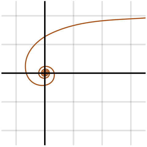
In the last episode of my column in Notices of the American Mathematical Society, we looked at a particle moving in an attractive central force whose strength is proportional to the inverse cube of the distance from the origin. Among other things, we saw that a particle moving in such a force can spiral in to the origin in a finite time. But that was classical mechanics. What about quantum mechanics?
Here things get more tricky. The uncertainty principle tends to prevent the particle from falling in to the origin. But when the attractive force is strong enough, the particle can still fall in. We can make up a theory where the particle shoots back out, but there are choices involved: we need to say how the particle changes phase when shoots back out. So there is not just a single theory, but many!
Why does the particle come back out? There are theories where it does not. In these theories, at least those studied so far, time evolution is nonunitary: that is, the probability of finding the particle somewhere or other does not stay equal to , because the particle simply disappears when it hits the origin. Here we focus on theories where time evolution is unitary and the particle comes back out. Many people have written about these, running into ‘paradoxes’ when they weren’t careful enough. Only rather recently have things been straightened out.
Let us dig into the details. In quantum mechanics, the Hilbert space of states of a particle in is . In a central force whose strength is proportional to , such a particle has a Hamiltonian of this form:
The first term describes the particle’s kinetic energy, while the second describes its potential energy: remember, taking the gradient of an inverse square potential gives an inverse cube force. I have set some constants to to remove irrelevant clutter, but we need the constant to say how strong the force is. When , the force is attractive.
In this game, analysis is paramount. We should interpret as a densely defined linear operator on . For this, we choose a dense linear subspace and treat as a linear map from to . Different choices of correspond to different physical assumptions: for example, assumptions about what happens when the particle falls into the origin.
To get unitary time evolution in quantum mechanics, we need the Hamiltonian to be self-adjoint. But adjoints of densely defined operators are tricky. Let us briefly recall how they work. Given a Hilbert space and a linear operator from a dense linear subspace to , we define to be the set of all for which there exist such that
If such a vector exists, it is unique, and it depends linearly on . Thus, for we define to be the vector with the above property. The adjoint of is then the linear operator . We say is self-adjoint if . We say that is essentially self-adjoint if it has a unique extension to a self-adjoint operator. If it does, this extension must be .
All this raises the question of whether the Hamiltonian for the inverse cube force law can be made self-adjoint with a suitable choice of domain. It turns out we can always do it, but sometimes in more than one way. There are three regimes:
. In this case we can start with the domain consisting of smooth functions that are compactly supported on minus the origin. The operator is unambiguously defined on this domain, and it is essentially self-adjoint.
. In this case is still well-defined on the domain , but it is not essentially self-adjoint. In fact, it admits more than one self-adjoint extension! However, is bounded below: there is a constant such that for all . Physically, this means that the particle’s energy is bounded below by . Mathematically, this implies that has a canonical choice of self-adjoint extension called the ‘Friedrichs extension’, with the smallest possible domain. But there is another canonical choice, the ‘Krein extension’, with the largest possible domain.
. In this case is well-defined on the domain , and it has more than one self-adjoint extension, but it is not bounded below.
These strange results demand explanation. For example, what is special about ? In classical mechanics, the energy of a particle in the inverse cube force ceases to be bounded below as soon as . Quantum mechanics is different. To get a lot of negative potential energy, the particle’s wavefunction must be peaked near the origin, but that gives it kinetic energy. The tradeoff is captured by Hardy’s inequality. This says that for any we have
This is why is bounded below when .
On the other hand, the constant in Hardy’s inequality cannot be improved, so if we can find with . Then we can use a remarkable property of the potential to show that is not bounded below. Namely, has a kind of symmetry under dilations. You can guess this by noting that both the Laplacian and have units of 1/length. Indeed, if you take any smooth function , dilate it by a factor of , and then apply , you get times what you get if you do these operations in the other order. This implies that if
we can dilate and get a function obeying the same equation with replaced by . Thus, as soon as can be negative, it can be made arbitrarily large and negative by choosing to be very small. Thus is not bounded below.
Next, what is special about ? This is more subtle. For any value of we can find spherically symmetric solutions of on that are nonzero and smooth. When , and only in this case, some of these solutions lie in . This dooms the chance of being essentially self-adjoint, because it implies . If were essentially self-adjoint would be self-adjoint, and it is easy to see that a self-adjoint operator cannot have as an eigenvalue.
When the operator has more than one self-adjoint extension from to some larger domain. To classify these we can use separation of variables, writing as a sum of a radial part and an angular part, assuming the angular dependence of is given by a spherical harmonic , and doing a change of variables to reduce to the ordinary differential operator
on the half-line . We can completely classify self-adjoint extensions of this differential operators from to larger domains; the answer depends on and . A choice of self-adjoint extension is a choice of boundary conditions at , and this says how the phase of an incoming wave changes as it reflects off the origin and bounces back. Finally, we can assemble the results for different spherical harmonics to classify self-adjoint extensions of .
There exist many self-adjoint extensions of that respect the rotational symmetry of the inverse cube force law, but for the extension must break the dilation symmetry discussed above. This is what physicists call an ‘anomaly’: a symmetry of a classical system that fails to be a symmetry of the corresponding quantum system. Intriguingly, for some even lower values of one can choose a self-adjoint extension that is symmetrical under a discrete subgroup of dilations. Determining precisely which values these are seems to be an open problem.
To explore this topic thoroughly, I recommend first this:
- S. Gopalakrishnan, Self-Adjointness and the Renormalization of Singular Potentials, B.A. Thesis, Amherst College, 2006.
then this:
- D. M. Gitman, I. V. Tyutin and B. L. Voronov, Self-adjoint extensions and spectral analysis in Calogero problem.
and finally this:
- J. Dereziński and S. Richard, On Schrödinger operators with inverse square potentials on the half-line, Ann. Henri Poincaré 18 (2017), 869–928.
The first is an excellent overview of problems associated to singular potentials, including the inverse cube force. The second delves into self-adjoint extensions of the ordinary differential operators mentioned above, and the third works them out with exquisite thoroughness.

Re: Quantum Mechanics of the Inverse Cube Force Law
The dilation argument for being bounded below is very nice.
The fact that the critical values of are and feels suspiciously simple, for some reason. I would have expected a somewhere in there.