The n-Category Café

We’ve seen that the category of tame species $\mathsf{FinSet}^{\mathsf{E}}$ has a lot of structure resembling that of the ring of formal power series $\mathbb{R}[[x]]$, but it’s richer because two tame species can have the same generating function. To dig deeper we need to understand that and exploit this analogy. But what do I mean exactly?

For starters, we can add and multiply species:

Addition. Given species $F, G : \mathsf{E} \to \mathsf{Set}$, they have a sum $F + G$ with

$$(F + G)(S) = F(S) + G(S)$$

where at right the plus sign means the disjoint union, or coproduct, of sets. Here I’ve said what $F + G$ does to objects $S \in \mathsf{FinSet}$, but it does something analogous to morphisms — figure it out and check that it makes $F + G$ into a functor! If $F$ and $G$ are tame, so is $F + G$, and

$$\widehat{F + G} = \widehat{F} + \widehat{G}$$

Multiplication. Given species $F, G : \mathsf{E} \to \mathsf{Set}$, I said last time that we can multiply them and get a species $F \cdot G$ with

$$(F \cdot G)(S) = \sum_{X \subseteq S} F(X) \times G(S - X)$$

Again, I’ll leave it to you to guess what $F \cdot G$ does to morphisms and check that $F \cdot G$ is then a functor. If $F$ and $G$ are tame, so is $F \cdot G$, and

$$\widehat{F \cdot G} = \widehat{F} \cdot \widehat{G}$$

Exercise 5. If you know about coproducts, you can show that $F + G$ is the coproduct of $F$ and $G$ in the category of species, $\mathsf{Set}^\mathsf{E}$, which we defined last time.

Exercise 6. If you know about products), you can show that $F \cdot G$ is not the product of $F$ and $G$ in the category of species. Thus, we often call it the Cauchy product. But if you know about symmetric monoidal categories, you can with some significant work show that the Cauchy product makes $\mathsf{Set}^\mathsf{E}$ into a symmetric monoidal category. For starters, this means that it’s associative and commutative up to isomorphism—but it means more than just that. (If you know about Day convolution, this can speed up your work.)

Now let’s think about addition and the Cauchy product together. We can check that

$$F \cdot (G + H) \cong F \cdot G + F \cdot H$$

and indeed addition and the Cauchy product give the category of species a structure much like that of a ring! It’s even more like a ‘rig’, which is a ‘rings without negatives’, since we can add and multiply species, but not subtract them. But all the rig laws hold, not as equations, but as natural isomorphism.

In fact the binary coproduct is just a special case of something called a colimit#Colimits), defined by a more general universal property. And the Cauchy product distributes over all colimits! We thus say the category of species is a ‘symmetric 2-rig’.

A bit more precisely:

Definition. A 2-rig is a monoidal category $(\mathsf{R}, \otimes, I)$ with all colimits, such that the tensor product $\otimes$ distributes over colimits in each argument. That is, if $\mathsf{D}$ is any small category and $F: \mathsf{D} \to \mathsf{R}$ is any functor, for any object $r \in \mathsf{R}$, the natural morphisms

$$\text{colim}_{i \in \mathsf{D}} \left( r \otimes F(i) \right) \quad \longrightarrow \quad r \otimes \left(\text{colim}_{i \in \mathsf{D}} F(i) \right)$$

$$\text{colim}_{i \in \mathsf{D}} \left( F(i) \otimes r \right) \quad \longrightarrow \quad \left( \text{colim}_{i \in \mathsf{D}} F(i) \right) \otimes r$$

are isomorphisms.

Definition. A symmetric 2-rig is a 2-rig whose underlying monoidal category is a symmetric monoidal category.

One can work through the details of these definitions and show the category of species is a symmetric 2-rig. But something vastly better is true. It’s very similar to the ring of polynomials in one variable!

Why is the ring $\mathbb{Z}[x]$, the ring of polynomials in one variable with integer coefficients, so important in mathematics? Because it’s the free ring on one generator! That is, given any ring $R$ and any element $r \in R,$ there’s a unique ring homomorphism

$$f: \mathbb{Z}[x] \to R$$

with

$$f(x) = r$$

To see this, note that the homomorphism rules force that for any $P \in \mathbb{Z}[x]$ we have

$$f(P) = P(r)$$

I claim that the 2-rig of species is similar: it’s the free symmetric 2-rig on one generator $X$. But what is this species $X$?

$X$ is the structure of ‘being a 1-element set’. What I mean is this: it’s the structure that you can put on a finite set $S$ in a unique way if $S$ has one element, and not at all if $S$ has any other number of elements. In other words:

$$X(S) = \left\{ \begin{array}{ccl} 1 & \text{if} & |S| = 1 \\ \emptyset & \text{if} & |S| \ne 1 \end{array} \right.$$

The name $X$ is appropriate because the generating function of this species is $x$:

$$\widehat{X} = \sum_{n \ge 0} \frac{|X(n)|}{n!} x^n = x$$

Here’s the big theorem, which I won’t prove here:

Theorem. The symmetric 2-rig of species, $\mathsf{Set}^\mathsf{E}$, is the free symmetric 2-rig on one generator. That is, for any symmetric 2-rig $\mathsf{R}$ and any object $r \in \mathsf{R}$, there exists a map of 2-rigs

$$f: \mathsf{Set}^\mathsf{E} \to \mathsf{R}$$

such that $f(X) = r$, and $f$ is unique up to natural isomorphism.

This result has a baby brother, too. First, note that the free ring on no generators is $\mathbb{Z}$. That is, $\mathbb{Z}$ is the initital ring: for any ring $R$ there exists a unique ring homomorphism

$$f: \mathbb{Z} \to R$$

This should make us curious about the free symmetric 2-rig on no generators. This is the category of sets, with its cartesian product as the symmetric monoidal structure.

Theorem. The symmetric 2-rig of sets, $\mathsf{Set}$, is the initial 2-rig. That is, for any symmetric 2-rig $\mathsf{R}$ there exists a map of 2-rigsar

$$f: \mathsf{Set} \to \mathsf{R}$$

which is unique up to natural isomorphism.

So we have a wonderful analogy:

The category of sets is to $\mathbb{Z}$ as the category of species is to $\mathbb{Z}[x]$.

This suggests that there’s a lot more one can do to ‘categorify’ ring theory — that is, to take ideas from ring theory and develop analogous ideas in 2-rig theory. And even better, it shows that a lot of combinatorics is categorified ring theory!

But let’s see how we can use this 2-rig business to count things. Let’s make up a species $B$ where a $B$-structure on a finite set is a way of the leaves of a rooted planar binary tree.

Here are some rooted planar binary trees:

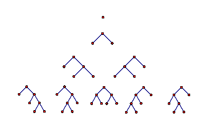
There’s 1 rooted planar binary tree with 1 leaf, 1 with 2, 2 with 3, 5 with 4… and so on.

I’ll draw lots of pictures to explain these trees and what it means to label their leaves by elements of a finite set, but the quickest definition is recursive, involving no pictures.

To put a $B$ structure on a finite set $S$, we either

• put an $X$-structure on it

or

• partition it into two parts $T$ and $S - T$ and put a $B$-structure on each part.

Remember, an $X$-structure on $S$ is the structure of ‘being a one-element set’. This handles the case of the binary tree with just one leaf.

We can state this recursive definition as an equation:

$$B(S) = X(S) + \sum_{T \subseteq S} B(T) \times B(T - S)$$

and we can express this more efficiently using the sum and Cauchy product of species:

$$B = X + B \cdot B$$

We can now use this to count $B$-structures on a finite set! By taking generating functions we get

$$\widehat{B} = x + \widehat{B}^2$$

or

$$\widehat{B}^2 - \widehat{B} + x = 0$$

This is a quadratic equation for the formal power series $\widehat{B}$, which we can solve using the quadratic formula!

$$\widehat{B} = \frac{1 \pm \sqrt{1 - 4 x}}{2}$$

Since the coefficients of a generating function can’t be negative, we must have

$$\widehat{B} = \frac{1 - \sqrt{1 - 4 x}}{2}$$

since the other sign choice gives a term proportional to $x$ with a negative coefficient. Using a computer we can see

$$\frac{1 - \sqrt{1 - 4 x}}{2} = x + x^2 + 2 x^3 + 5 x^4 + 14 x^5 + 42 x^6 + 132 x^7 + 429 x^8 + 1430 x^9 + 4862 x^10 + 16796 x^11 + \cdots$$

Remember

$$\widehat{B} = \sum_{n \ge 0} \frac{|B(n)|}{n!} x^n$$

so we get

$$\frac{|B(0)|}{0!} = 0$$

$$\frac{|B(1)|}{1!} = 1$$

$$\frac{|B(2)|}{2!} = 1$$

$$\frac{|B(3)|}{3!} = 2$$

$$\frac{|B(4)|}{4!} = 5$$

$$\frac{|B(5)|}{5!} = 14$$

and so on. The factorials arise because there are $n!$ ways to label the leaves of a planar binary tree with $n$ leaves by elements of $\{0, \dots, n-1\}$ . The interesting part is the sequence

$$0, 1, 1, 2, 5, 14, \dots$$

These give the number of planar binary trees with $n$ leaves! They’re called the Catalan numbers.

Exercise 7. Use your mastery of Taylor series to show that

$$\frac{1 - \sqrt{1 - 4 x}}{2} = \sum_{n \ge 0} \frac{2^{n-1} (2n-3)!!}{n!} x^n$$

so

$$\frac{|B(n)|}{n!} = \frac{2^{n-1} (2n-3)!!}{n!}$$

Let’s check this for $n = 4$:

$$\frac{2^{4-1} (2\cdot 4-3)!!}{4!} = \frac{8 \cdot 5!!}{4!} = \frac{8 \cdot 5 \cdot 3 \cdot 1}{1 \cdot 2 \cdot 3 \cdot 4} = 5$$

which matches how there are 5 rooted planar binary trees with 4 leaves!