The n-Category Café

The category $Span(C)$

The category $Span(C)$ is built from the category $C$ by considering diagrams of the form $L \leftarrow A \rightarrow R$, where $A$ is the apex of the span, and $L, R$ are the base of the span. The ordering of left and right is important when we describe the composition of spans. Formally, the objects of $Span(C)$ are the objects of $C$. The arrows of $Span(C)$ are from $A$ to $B$ are spans ($A \xleftarrow{f} X \xrightarrow{g} B$).

Now, a natural question is to ask how one composes spans. We compose spans by taking their pullback. Consequently, the category $Span(C)$ only exists if $C$ has all pullbacks. The composition of a span ($A \xleftarrow{f} X \xrightarrow{g} B$) with another ($B \xleftarrow{h} Y \xrightarrow{k} C$) is given by the pullback $X \times_B Y$ with the associated diagram:

Some examples of spans follows:

• First, as mathematicians, we are honor-bound to give the trivial example ($A \xleftarrow{\rm id} A \xrightarrow{\rm id} A$) is the identity span on the object $A$.

• Next, any arrow $f: A \to A'$ can be considered as a span on the left ($A' \xleftarrow{f'} A \xrightarrow{\rm id} A'$), or as a span to the right ($A \xleftarrow{\rm id} A \xrightarrow{f} A'$). Note that these define a pair of functors from $C$ to $Span(C)$.

A prototypical example of spans is the span of two finite sets. Suppose we have two sets $A, B$, and we wish to describe the set of ways to go from $A$ to $B$ (where we think of $A$ and $B$ as abstract locations). In such a case, we need a set $S$, which describes the set of ways to get from $A$ to $B$, and morphisms $\pi_A: S \to A$, $\pi_B: S \to B$ that gives us the start and end position of a path from some element of $A$ to some element of $B$.

Remark The pullback, and thus the composition of spans, is only unique up to isomorphism. Hence, $Span(C)$ is only a proper category if the morphisms are taken to be the isomorphism classes of spans.

The category $Graph$ of directed multigraphs

There are many slightly different notions of a graph in the literature. For our exposition, we will focus on the category of directed multigraphs. Intuitively, this means that we have vertices (states of an automata) and edges (transitions). There can be multiple edges between a pair of vertices (there are multiple ways to transition from one state into another).

Formally, a multigraph is given by a vertex set $V$, a set of edges $E$ and a pair functions $s, t: E \to V$ which denote the source and target of the edge. We will denote a graph as $G \equiv (V, E)$ as a pair of its vertex and edge set. We denote $V(G)$ for the vertex set of $G$, and $E(G)$ for the edge set of $G$.

The objects of the category $Graph$ are these directed multigraphs. The arrows of this category are multigraph morphisms.

A morphism $f: G \to H$ in this category is given by two set valued functions $f_V: V(G) \to V(H)$ which maps vertices, and $f_E: E(G) \to E(H)$ which maps edges, under the condition that the images of the edges are consistent with the images of the vertices. That is, for all $e \in E(G)$, $s(f_E(e))=f_V(s(e))$ and $t(f_E(e))=f_V(t(e))$. Said differently, the above condition means that edges must preserve adjacency.

Remark A more concise way to define the above construction is as the presheaf category $[Arr^{op}, Set]$, over the diagram $Arr=(V \xrightarrow{s, t} E)$, whose objects are functors $G: Arr^{op} \to Set$ and morphisms are natural transformations.

The (co)limits of $Graph$

The category of graphs has products $X \times Y$, which is computed pointwise: $E(X \times Y)=E(X) \times E(Y)$ and $V(X \times Y)=V(X) \times V(Y)$. Similarly, it has coproducts $X+Y$, also computed pointwise. $Graph$ can thus be made into a cartesian monoidal category $(Graph, \otimes=\times, I=(\star \to \star))$ or a cocartesian category $(Graph, \otimes=+, I=\emptyset)$.

The pullback of a diagram of graphs $X \xrightarrow{f} Z \xleftarrow{g} Y$, written $X \times_Z Y$, intuitively performs a pullback along the vertices and the edges. Formally, it is a graph $X \times_Z Y$ whose vertex set is the pullback of the vertices: $V(X \times_Z Y) \equiv \{ (v, v') : v \in V(X), v' \in V(Y), f_V(v) = g_V(v') \}$, and whose edge set is the pullback of the edges: $E(X \times_Z Y) \equiv \{ (e, e') : e \in E(X), e' \in E(Y), f_E(e) = g_E(e') \}$.

The pushout dualizes the above construction. Intuitively, it glues two graphs along a third one. Formally, the pushout of a diagram of graphs $X \xleftarrow{f} Z \xrightarrow{g} Y$, written $X +_Z Y$, is a quotient $X+Y/\sim$ by the equivalence generated by $f_V(v) \sim g_Z(v), v \in V(Z), f_E(e) \sim g_E(e), e \in E(Z)$.

Remark Seeing $Graph$ as the functor category $[Arr^{op}, Set]$, $Graph$ automatically derives the above limits and colimits from $Set$. The (co)limits are then computed pointwise.

Parallel composition of automata with $Span(Graph)$

At this stage, we have the machinery necessary to add labels onto our graph edges, by means of exploiting $Span(Graph)$, which is a category as $Graph$ has pullbacks. $Span(Graph)$ is a symmetric monoidal category with the monoidal product deriving from the cartesian monoidal structure on $Graph$.

In our case, for automata, we focus on the situation where the graphs at the base are graphs with a single vertex and many edges. These edges are thought of as transition labels. Formally, for a given set of labels $A$, we create the graph $\mathcal{E}(A) \equiv (\star, A)$.

An automaton is then a span $\mathcal{E}(A) \xleftarrow{f} G \xrightarrow{g} \mathcal{E}(B)$. The states of the automaton are the vertices $V(G)$ and the transitions the edges $E(G)$. By definition, each transition $e \in E(G)$ maps to some edge $a=f_E(e) \in E(\mathcal{E}(A))=A$ and some edge $b=g_E(e) \in E(\mathcal{E}(B))=B$. We denote this diagramatically as a label $a/b$ on the transition.

When composing spans $\mathcal{E}(A) \leftarrow G \rightarrow \mathcal{E}(B)\leftarrow G' \rightarrow \mathcal{E}(C)$, we get $\mathcal{E}(A) \leftarrow G \times_{\mathcal{E}(B)} G' \rightarrow \mathcal{E}(C)$. This composition can be interpreted as synchronized parallel computation. The pullback contains all vertices $V(G) \times V(G')$, meaning that the state $(v,v')$ of the composed automaton is a product of both a state $v$ of automaton $G$ and a state $v'$ of automaton $G'$. For the transitions, however, only the edges $(e, e')$ that have the same $B$ label survive. This can be interpreted as a requirement that automata $G$ and $G'$ communicate and can only transition when their $B$ signal agrees.

Sequential composition of automata with $Copan(Graph)$

In the exact same way that $Span(Graph)$ provides us with parallel composition, dualising the construction to $Cospan(Graph)$ gives us sequential composition. This is a category whose objects are graphs, morphisms are cospans $X \rightarrow Z \leftarrow Y$ of graphs and composition is given by pushout, which exist for $Graph$. $Cospan(Graph)$ is a symmetric monoidal category due to the cocartesian monoidal structure on $Graph$.

For a set $A$, define the graph $\mathcal{V}(A)\equiv(A,\emptyset)$ to contain no edges. Then a cospan $\mathcal{V}(A) \to G \leftarrow \mathcal{V}(B)$ can be interpreted as an automaton with states $V(G)$ and edges $E(G)$ having $A$ input states, with each $a \in A$ corresponding to a state $v \in V(G)$, and similarly $B$ output states.

A composition of cospans $\mathcal{V}(A) \rightarrow G \leftarrow \mathcal{E}(B)\rightarrow G' \leftarrow \mathcal{E}(C)$ of automata yields a new automaton $\mathcal{V}(A) \rightarrow G +_{\mathcal{V}(B)} G' \leftarrow \mathcal{V}(C)$. This composition can be thought of as sequential computation, as the state of the composed automaton is either a state $v$ of $G$ or a state $v'$ of $G'$, where we glue toghether output and inputs states, because we make the equivalence that $v \sim v'$ if $v$ corresponds to an output $b \in B$ that corresponds as an input to $v'$.

Wiring in Span(Graph)

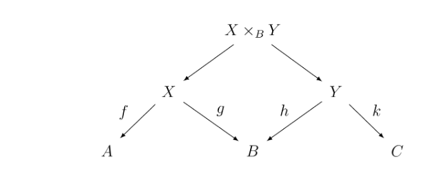
Composition in Span(Graph) allows one to compose spans $X \leftarrow G \rightarrow Y \leftarrow G' \rightarrow Z$ into a span between $X$ and $Z$, while the tensor product of spans $X \leftarrow G \rightarrow Y, X' \leftarrow G' \rightarrow Y'$ yield a span between $X \times X'$ and $Y \times Y'$. However, to allow for more flexible compositions, such as the composition of spans $X \leftarrow G \rightarrow Y, X \leftarrow G' \rightarrow Z$ into a span between $X$ and $Y \times Z$, one needs morphisms to connect multiple copies of $X$. In a string diagram of $Span(Graph)$ this looks like:

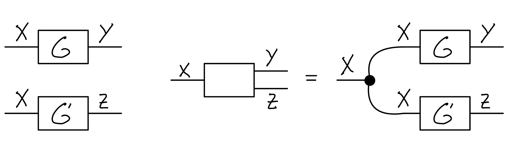
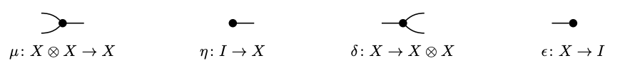
As automata, this corresponds to a synchronization between the parallel processes $G$ and $G'$, so that they can transition when their left $X$ transition is equal. Generally, such connectors between parallel $X$ interfaces of automata are given by a Frobenius monoid on $X$, which consists of the following spans: - $X \times X \xleftarrow{\Delta} X \xrightarrow{\rm id} X$, giving $\mu_X : X \times X \to X \in Span(Graph)$ - $I \xleftarrow{!} X \xrightarrow{\rm{id}} X$, giving $\eta_X : I \to X \in Span(Graph)$ - $X \xleftarrow{\rm{id}} X \xrightarrow{\Delta} X \times X$, giving $\delta_X : X \to X \times X \in Span(Graph)$ - $X \xleftarrow{\rm{id}} X \xrightarrow{!} I$, giving $\epsilon_X : X \to I \in Span(Graph)$

where we use the following morphisms in $Graph$: - $!: X \to I$, where the monoidal unit $I$ is the terminal graph with a single vertex and single loop. - $\Delta: X \to X \times X$ that is the identity on the components. Concretely on graphs, it maps vertex $v$ to $(v,v)$ and edge $e$ to $(e,e)$.

These are written as string diagrams in $Span(Graph)$ [figs from Fong & Spivak 2019]

It can be shown that these obey the commutative monoid axioms

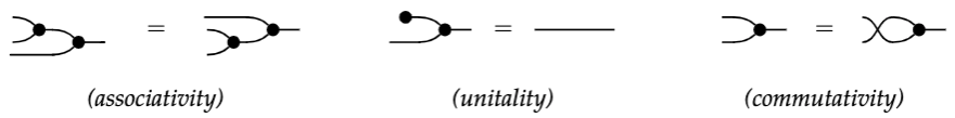
the cocommutative comonoid axioms

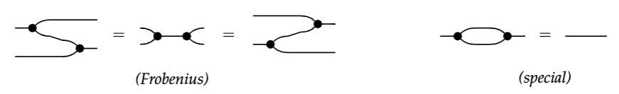
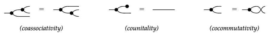and the Frobenius and special axioms

Definition. A tuple $(X, \mu_X, \eta_X, \delta_X, \epsilon_X)$ of such maps satisfying these axioms is called a special commutative Frobenius monoid.

Theorem. [Fong & Spivak 2018] Given a special commutative Frobenius monoid $(X, \mu_X, \eta_X, \delta_X, \epsilon_X)$, for two non-negative integers $m, n$, any map $X^{\otimes m} \to X^{\otimes n}$ composed of $\mu_X, \eta_X, \delta_X, \epsilon_X$ and the swap $\sigma_X$, whose string diagram is connected, equals the spider morphism $s_{n,m}$ given by

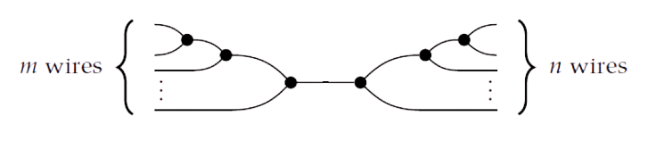
which is also written as

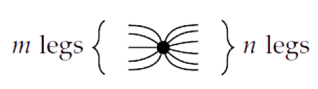
If a special commutative Frobenius monoid exist for all objects in a category and the Frobenius monoid for tensor products $X \otimes Y$ are composed of the Frobenius monoid of the objects $X$ and $Y$, then the category is called hypergraph category [Fong & Spivak 2019]. String diagrams of such categories can be interpreted as a hypergraph. A hypergraph is a graph in which the edges connect an arbitrary number of nodes. In this case, the spans are the nodes of the hypergraph and the spider morphisms form the hyperedges.

Remark The fact that $Span(Graph)$ is a hypergraph category relies on the fact that $Graph$ is a Cartesian category, a symmetric monoidal category whose tensor product is a categorical product and whose unit is terminal. Hence, for any Cartesian category $C$, $Span(C)$ is a hypergraph category. The spans in the Frobenius monoids are constructed similarly from the diagonal morphisms $\Delta: X \to X \times X$ and terminal maps $! : X \to I$.

Wiring in Cospan(Graph)

Similar to $Span(Graph)$, $Cospan(Graph)$ also forms a hypergraph category in which each object is equiped with a spider morphism. Recall that $Graph$ is a symmetric monoidal category with as tensor product $\otimes$ the disjoint union $+$ of graphs, which is a coproduct, and its unit is $I$, the initial graph $\emptyset$, which contains no edges and vertices. As such, it is equiped with a codiagonal map $\nabla: X + X \to X$, which is the identity on each part, and an initial map $!: I \to X$. For any graph $X$, one can construct the following cospans, constituting a special Frobenius monoid: - $X + X \xrightarrow{\nabla} X \xleftarrow{\rm id} X$, giving $\mu_X : X+X \to X \in Cospan(Graph)$ - $I \xrightarrow{!} X \xrightarrow{\rm{id}} X$, giving $\eta_X : I \to X \in Cospan(Graph)$ - $X \xrightarrow{\rm{id}} X \xleftarrow{\nabla} X \otimes X$, giving $\delta_X : X \to X \otimes X \in Cospan(Graph)$ - $X \xrightarrow{\rm{id}} X \xleftarrow{!} I$, giving $\epsilon_X : X \to I \in Cospan(Graph)$

Remark In more generality, for any cocartesian category $C$ - a symmetric monoidal category whose tensor product is a coproduct and unit is initial - $Cospan(C)$ is a hypergraph category.

Feedback via traces

Some automata may also want to synchronize their parallel left and right interfaces (in the case of $Span(Graph)$) or their sequential top and bottom interfaces (in the case of $Cospan(Graph)$). In either case, the hypergraph structure provides for this in the following way:

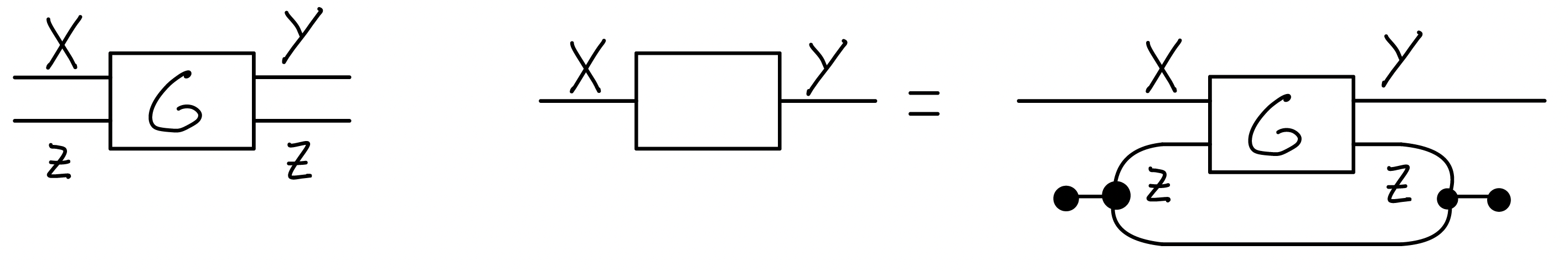
Hence, every hypergraph category $H$ is traced monoidal category, which are categories which provide a notion of feedback by providing for all objects $X, Y, Z$, a tracing map: $$Tr^Z_{X,Y} : H(X \otimes Z, Y \otimes Z) \to H(X, Y)$$ satisfying some coherence axioms.

Timing

A path in a directed graph is a sequence of edges $(e_0, e_1, ...)$ such that the tail node of edge $e_i$ equals the start node of edge $e_{i+1}$. In the context of an automaton, a path is called a behaviour. The automaton can be interpreted as a discrete time system, in the simplest case by saying that each edge has time duration 1, so that the duration of a behaviour equals the length of the path. Note that this notion of time is imposed as an interpretation, while the underlying model remains unchanged.

As an example, we will construct a clock by parallel composing automata that cycle with frequency 1, 60, 60 and 24. We define one parallel interface $X = \{s, \epsilon,\}$, corresponding to taking a step or remaining idle. We define an automaton $T$ with left interface $!= \{\star\}$ and right interface $X$ with one node and one edge: $1 \xrightarrow{\star/ s} 1$. This automaton sends a tick to the right at each step. Also, for any natural number $t$, we define automaton $G_t$ with left and right interface $X$:

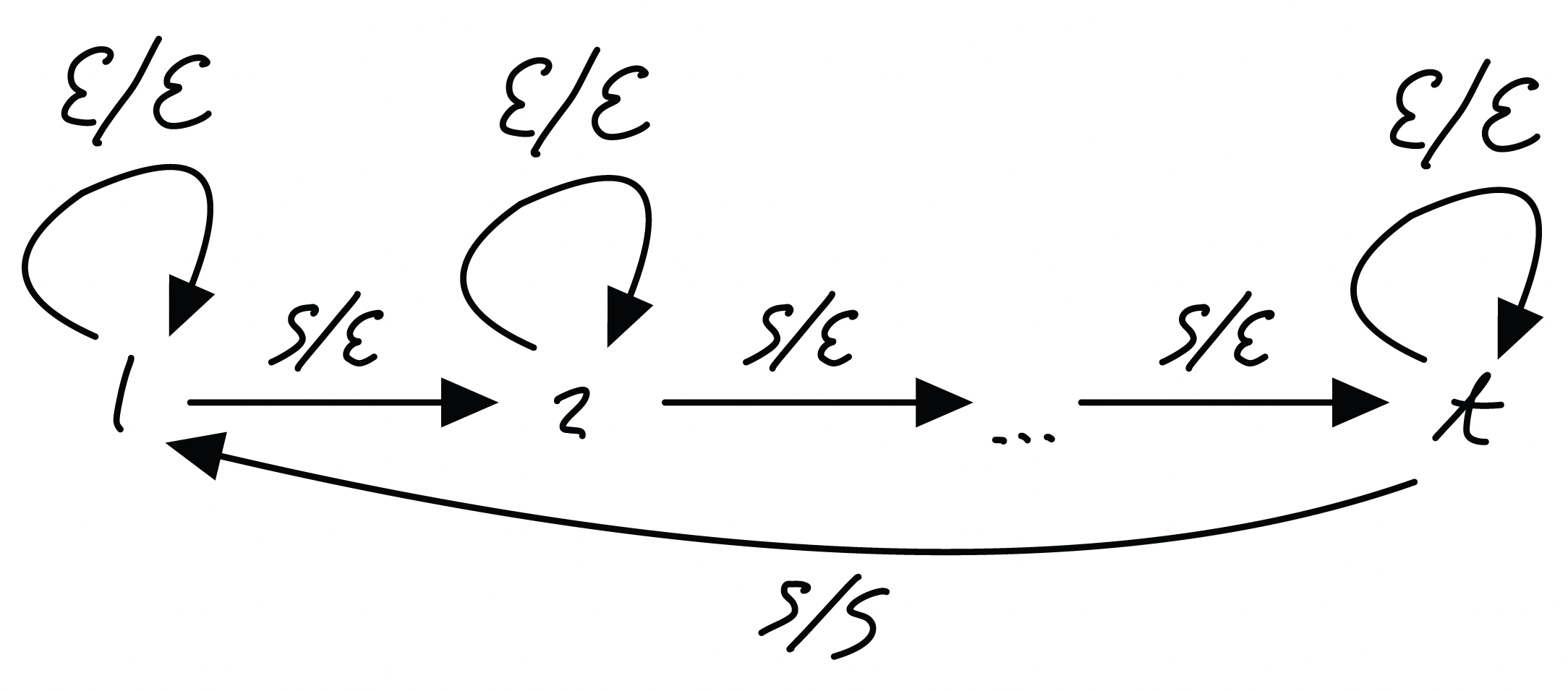
Whenever $G_t$ receives a tick from the left, it ticks itself. After $t$ ticks, it sends a tick to the right.

If we compose these automata as:

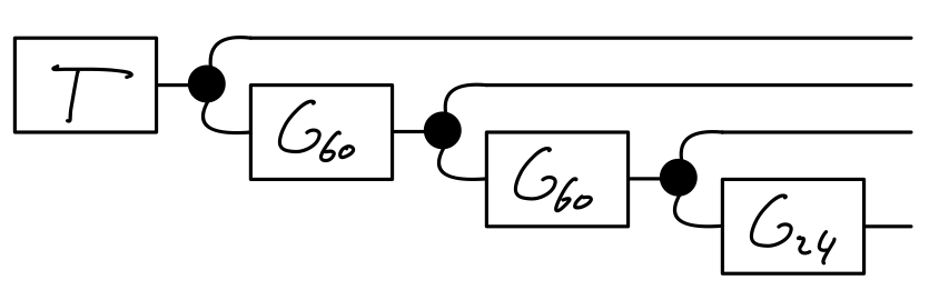
We get a unit interface on the left and interface $X \times X \times X \times X$ on the right. Its only behaviour is a single cycle of duration $1 \cdot 60 \cdot 60 \cdot 24$. The right labels are $s$ on the first position on each step, $s$ on the second position every 60 steps, $s$ on the third position every $60 \cdot 60$ steps and $s$ on the fourth position every $60 \cdot60 \cdot 24$ steps. We have built a clock.

References

• Baez, John C. “Spans in quantum theory.” Keynote talk at Deep Beauty: Mathematical Innovation and the Search for an Underlying Intelligibility of the Quantum World, Princeton University
• Alessandra Cherubini, Nicoletta Sabadini, Robert F. C. Walters: Timing in the Cospan-Span Model. Electron. Notes Theor. Comput. Sci. 104: 81-97 (2004)
• Brendan Fong and David I. Spivak. 2019. “Hypergraph Categories.” Journal of Pure and Applied Algebra 223 (11): 4746-77.
• Brendan Fong and David I. Spivak. 2018. “Seven Sketches in Compositionality: An Invitation to Applied Category Theory.”