Graphical Regular Logic
Posted by John Baez
.")
guest post by Sophie Libkind and David Jaz Myers
This post continues the series from the Adjoint School of Applied Category Theory 2019.
Graphical Regular Logic
guest post by Sophie Libkind and David Jaz Myers
This post continues the series from the Adjoint School of Applied Category Theory 2019.
Now that we have self-driving cars and talking watches, holographic data analysis should be the next innovation inspired by Hollywood spy films. Think of when Tom Cruise in Minority Report shuffles information around a 3D screen. As a step towards this future, Fong and Spivak formulated a graphical system for doing regular logic in their paper Graphical Regular Logic. You can see Spivak give a talk about it here. This visual knowledge representation system has the potential to be an intuitive user-interface for regular logic. It would allow laypeople to harness the power of regular logic without the clunkiness of the formal language.
The road from regular logic to graphical regular logic has two major stops: regular categories and regular calculi.
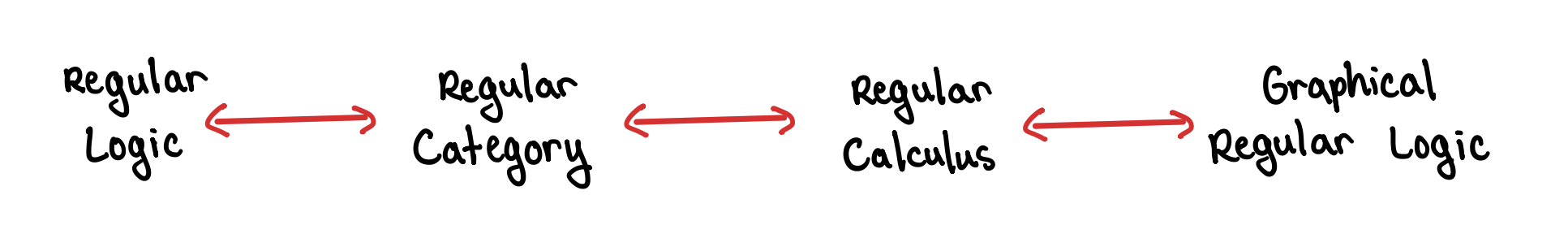
In this post, we’ll start on the right with graphical regular logic and work our way leftwards to regular categories.
Graphical Regular Logic: A User’s Guide
Graphical Regular Logic is meant to be broadly applicable and easy-to-use. So in this user’s guide we will apply it to something as non-mathy as a neighborhood watch program that is run by beings as gibberishy as a clan of minions.
Building blocks
When we imagine the headquarters of the neighborhood watch
program, there’s a big screen with glowing blue dots to
move, connect, and zoom in and out of. In graphical regular
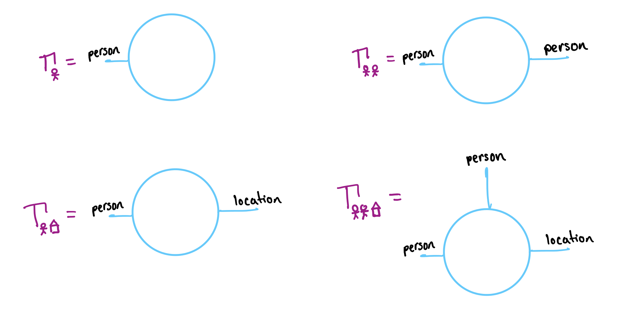
logic, these orbs are called shells. A shell has finitely many ports
labeled with a type and wires can connect ports of the same
type. In the neighborhood watch program, we care about types
like person and location and use shells like the
following.
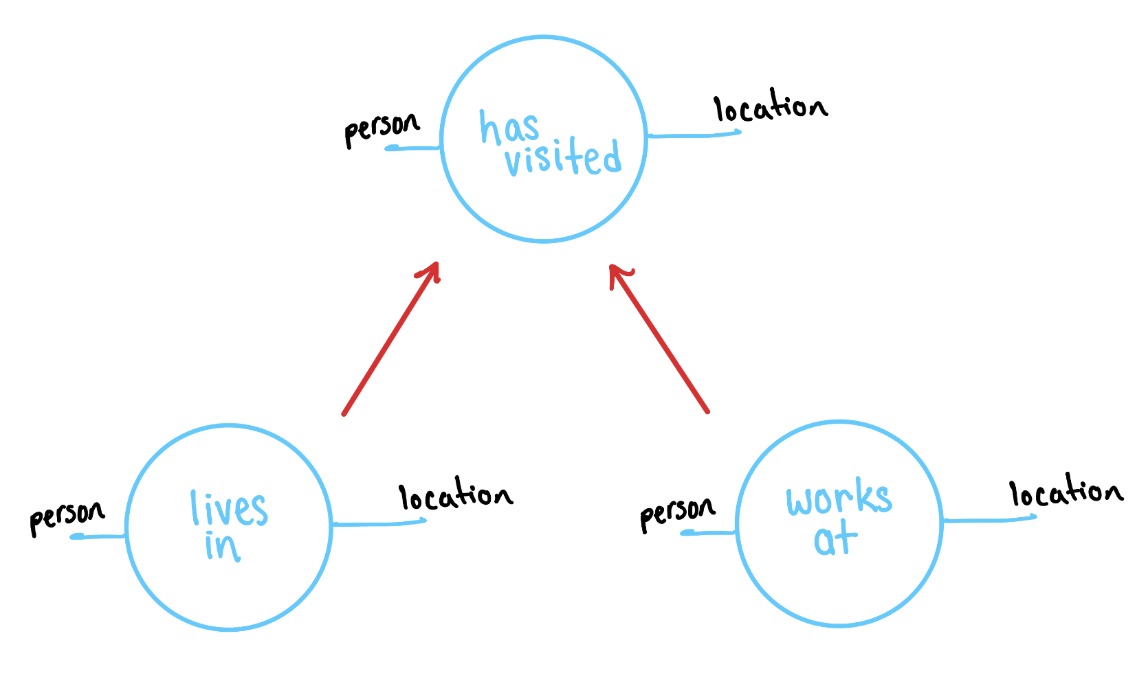
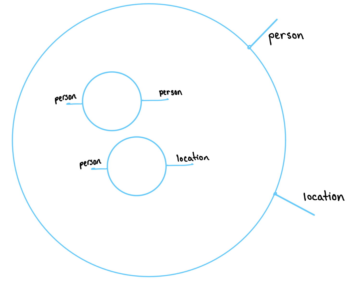
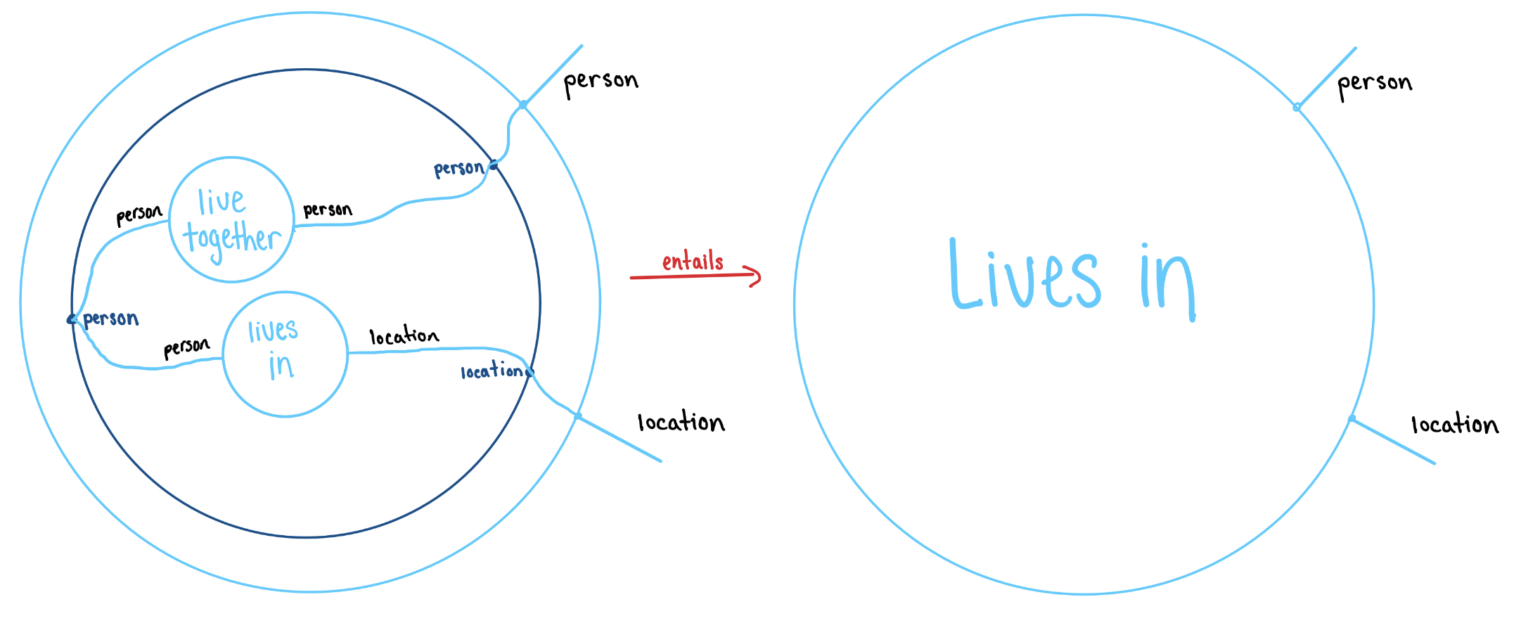
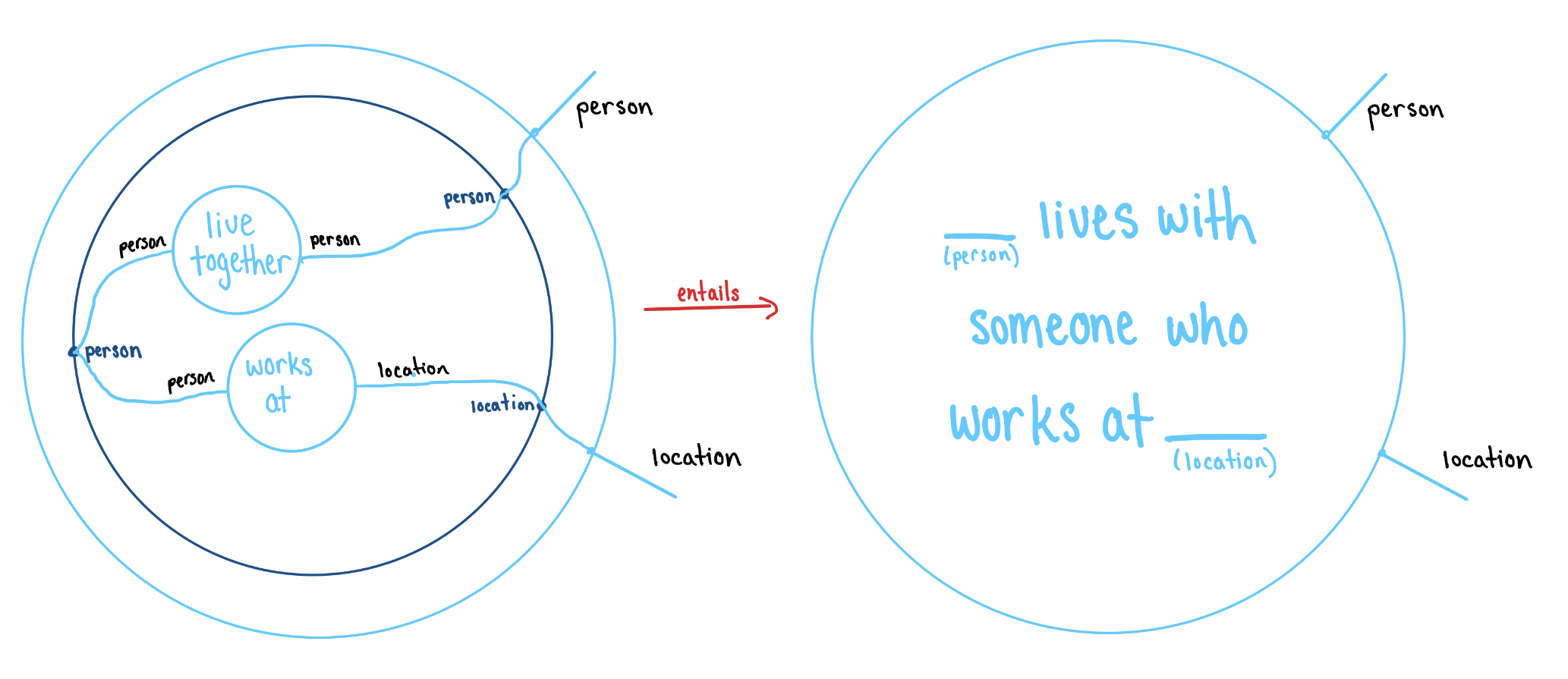
A shell is the foundation for talking about a relationship between the types labeled on the ports. A relationship between a person and a location (more formally a predicate in context ) is like a Madlibs with a blank space for a person and a location:
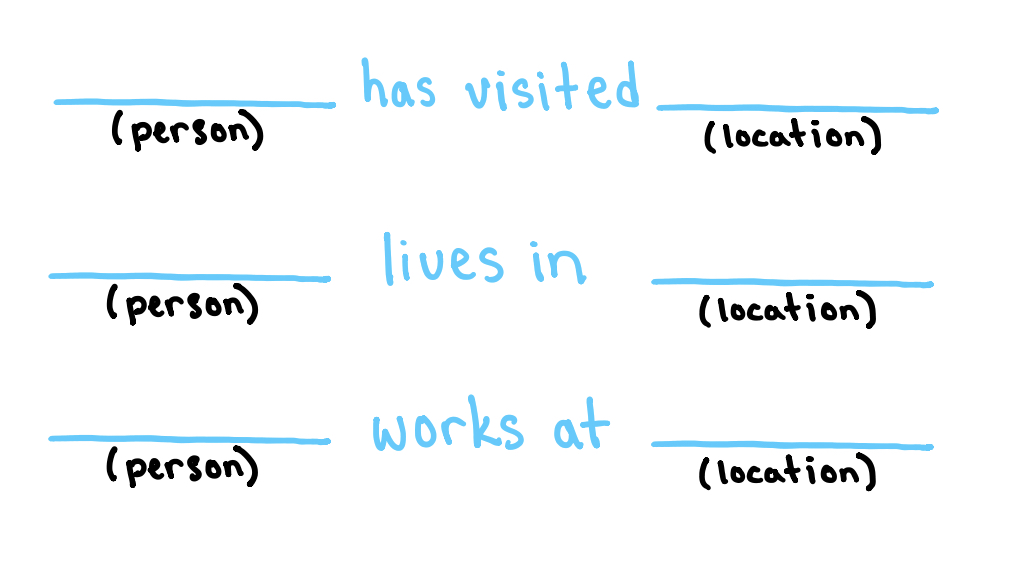
To represent such a relationship, we take a shell with a port for each blank space and fill the shell with the corresponding predicate.
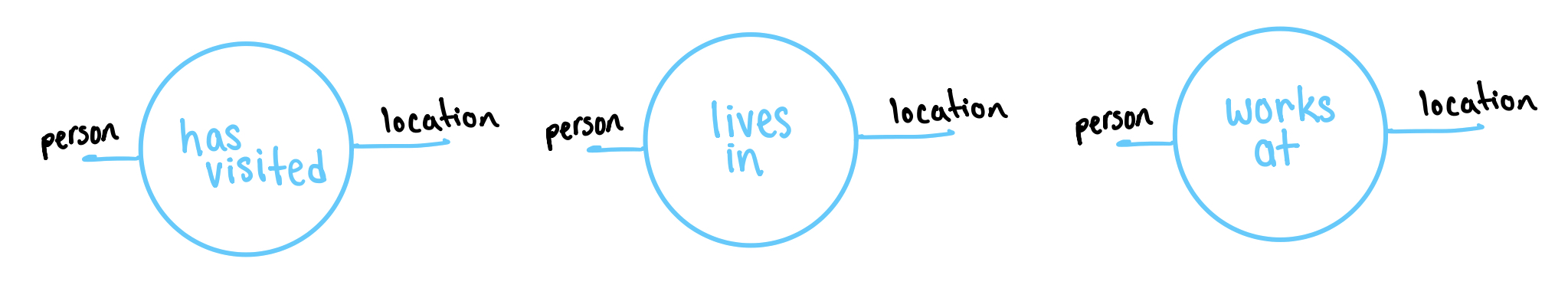
We would read the right cell as “There exists a person and a location such that works at ”. Every shell represents a possible relationship between the wires coming out of it. There is no implied directionality on these wires.
Operations
Now comes the fun part where we really get to feel like Tom Cruise. How do we manipulate the filled shells in a way that reflects logical moves?
Operation 1: Substitution
The most basic operation is to substitute one filled shell for another. If someone lives in a location, then it’s also true that they have visited that location. Therefore, if we see the filled shell corresponding to (person) lives in (location) then we should be able to replace it with the filled shell corresponding to (person) has visited (location). The red arrows below indicate when we can substitute one filled shell with another.
In general, we are allowed to substitute in the midst of a more complicated diagram.
Operation 2: Zooming out
Sometimes we want a coarser view of the neighborhood, so we will zoom out and blur two shells together. For example, suppose we have two relationships:
- Bob works at Gru’s house
- Edith has a roommate
And we want to turn them in to one relationship:
- Bob works at Gru’s house and Edith has a roommate
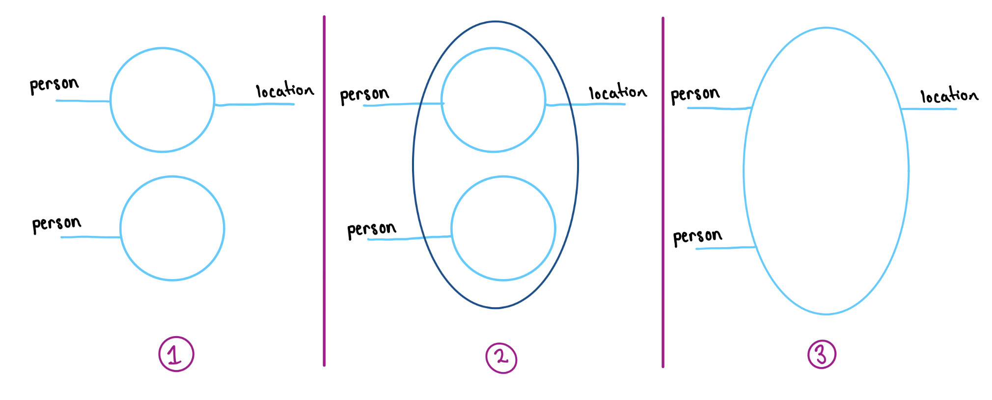
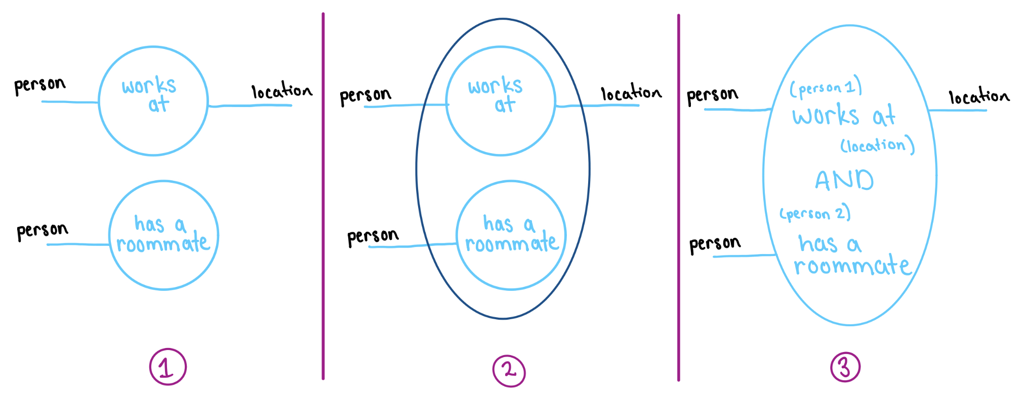
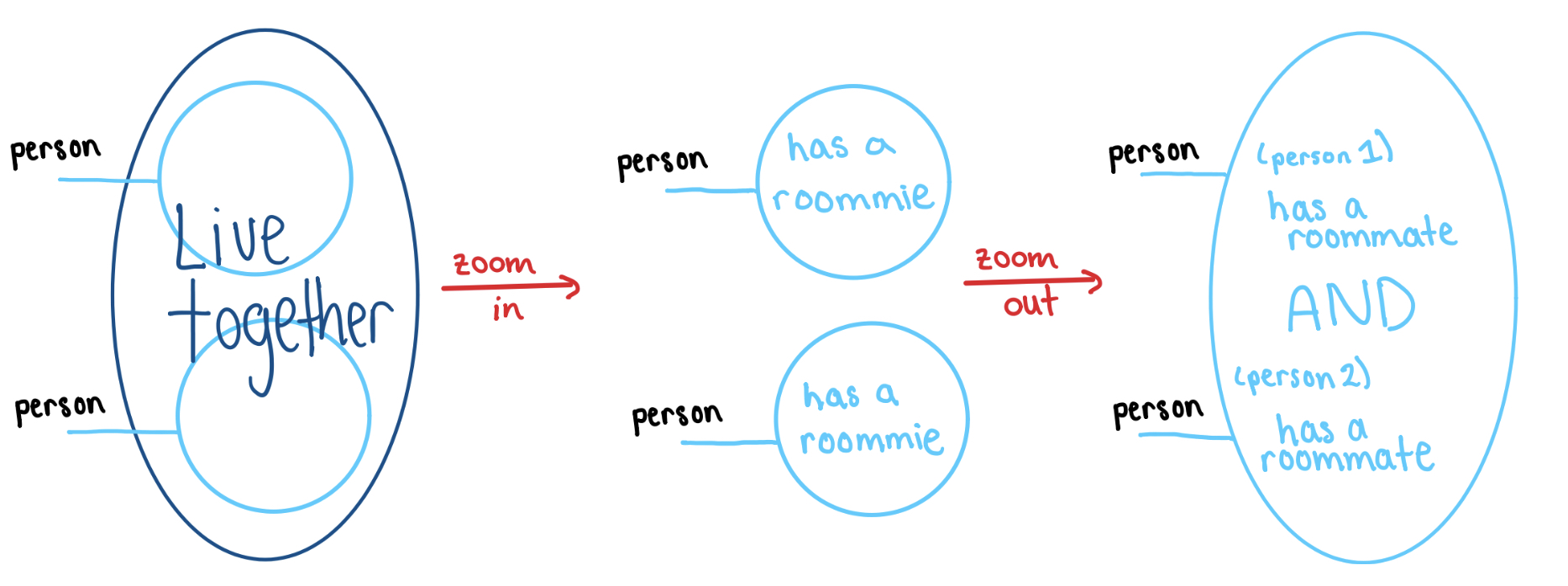
So we start with a relationship between a person and a location and a relationship on one person. And we want to transform these into one relationship about two people and a location. This process is called trench coating and goes as follows: (1) stack the two shells, (2) enclosed them in a trench coat, (3) ignore the coat’s interior.
At last the true purpose of this example comes to light:

Now filling the inner shells with predicates, determines a predicate for the trench coat in a way that corresponds with logical AND.
We will discuss this parallel more deeply when we show how to put a logic on the graphical calculus.
Operation 3: Zooming in
If we can zoom out, then we should also be able to zoom in to get a more fine-grained view of the neighborhood. Suppose we have a predicate which fills a trench coat. Then it defines a predicate on the inner shells by a process called dotting off.
Note that zooming in and out do not compose to the identity. In fact, in the next section we will show that they are adjoint operations.
Operation 4: Connecting Shells
To really tell a story about the neighborhood we need to be able to combine information and build complicated relationships out of the basic ones. For example, suppose we have two relationships:
- Agnes lives with Margo
- Margo lives in Gru’s house
And we want to derive the relationship:
- Agnes lives in Gru’s house
Step 1 Draw the shells corresponding to the input, inside of the shell corresponding to the output
Step 2 Draw an intermediate shell labeled with ports for the wires to attach through.
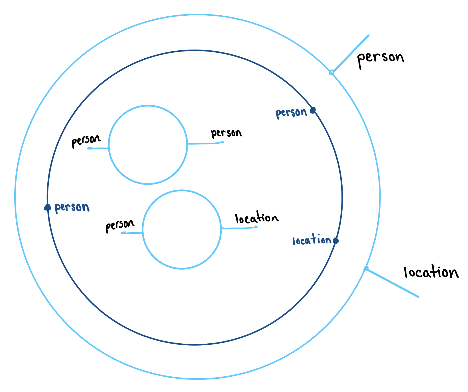
Step 3 Connect the wires.
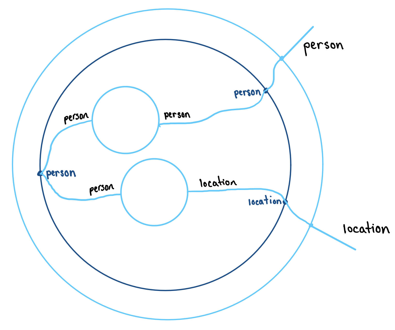
Once we have hooked up shells, any choice of predicates for the inner shells defines a relationship for the outer shell. In the example above, we have the entailment:
However if we fill the inner shells differently, we may get a different filling for the outer shell.
We would read the bottom left diagram as “There exists a person , a person and a location such that lives with and works at ”.
With these four operations, we can visually represent any deduction in regular logic. Next, we give a taste of how a graphical calculus presents a regular logic.
Putting a Logic on a Graphical Calculus
Before we dive into the particular relationship between the graphical calculus and regular categories, let’s take a little bit to dwell on some abstract ruminations.
Lawvere divides logic into two opposing modes: subjective and objective.
- Subjective logic is the logic we use to reason with – the syntax and the rules of inference. For example, the axioms of a boolean algebra.
- Objective logic is the logical arrangement of the objects we are interested in studying. For example, the power set of a given set.
We use the subjective logic to describe and reason about the objective logic at hand. This gives us a transformation which is sometimes called semantics from subjective to objective reasoning. For example, we can use the axioms of a boolean algebra to reason about the subsets of a given a set.
In nice cases, we can “objectify” our subjective logic by freely generating objective situations of our syntax. By stretching what we mean by syntax, we can also build subjective logics out of our objective situations. If everything goes perfectly, these two processes are inverse. A case where everything does go perfectly is Seely’s equivalence between first order (constructive) theories and hyperdoctrines, where the subjective first order constructive logic is interpreted into the objective logic of a hyperdoctrine.
In the situation at hand, the graphical calculus is our subjective logic for dealing with the objective logic of a regular category. We would like to put a logic back on our calculus – that is, build a regular category from a graphical calculus. However, we can’t do it with the pictures alone; we have to give a way for the pictures to mean something. How should we go about this?
Ajax Functors
The objects under consideration in predicate logic are the parts of a domain of discourse. The association of each object to its order of parts gives something akin to a hyperdoctrine. A hyperdoctrine is just an axiomatization of this association for first order constructive logic. We need something like this to add meaning to our pictures.
But hyperdoctrines are notoriously complex; they have a number of axioms that on a first read seem unmotivated (or, at least, they seemed that way to us). While they all turn out to directly correspond to features of the logic being modeled, it would be nice to have a more basic, conceptual axiomatization from which the desired properties follow. In the case of regular logic—the logic of “true”, “and”, and “exists”—David and Brendan find this conceptual axiomatization in the form of ajax functors. The definition of an ajax functor is not terribly complicated, but to understand why it does what we want takes a bit of work. So we’ll meander our way to the definition.
Regular logic is the logic of “truth”, “and” and “exists” – let’s bring them into the ajax frame in that order. Our ambient setting will be the category of ordered sets and order preserving maps. In fact, we will think of this as a 2-category where the arrows between order preserving maps are dominations , that is, (since we are thinking logically, I’ll denote the order relation by , which you can read as entails if you like). If you are familiar with enriched category theory, this is the 2-category of Boolean-enriched categories.
“Truth”, or , in an order theoretic sense, is the most general proposition. It has a mapping-in property; namely, from any proposition , one can infer . If is our ordered set of propositions and entailments, then would be an order preserving function from the terminal order. To say that has the universal property we expect, we can ask that be right adjoint to the terminal functor . In other words, we ask that that the top holds if and only if the bottom holds
where is our ordering and is the unique element of . Since per the axioms of an ordering, always, we always have that , as we wanted.
“And”, or , in an order theoretic sense, is the meet of two elements. The proposition is the most general proposition which proves both and . Its mapping in property can be expressed by
or, in other words, that is right adjoint to the diagonal map .
Now, it won’t come as a surprise that “truth” and “and” together form a monoid, but we can give a slick proof of this knowing that they are right adjoints. This is because and give the structure of a comonoid and taking right adjoints is contravariantly functorial. Monoids like this are common enough that we have a name for them:
Definition: In a monoidal 2-category, an adjoint monoid is a monoid whose unit and multiplication are right adjoints.
We just saw that all meet semi-lattices are adjoint monoids in the 2-category of orders, but we can flip the argument on its head to see that every adjoint monoid is a meet semi-lattice as well. This is because the 2-category of orders is cartesian, and in a cartesian category every object has a unique comonoid structure given by and . Since the left adjoints of the structure maps of an adjoint monoid form a comonoid, the right adjoints must be the top and meet.
“Exists” is a quantifier, and quantification is all about changing the domain of discourse. So we can’t really talk about “exists” without bringing in a system of domains of discourse, and this means bringing in a regular category. Let’s get back to regular categories now. A regular category is a category in which we can use the logic of “truth” (a terminal object), “and”, (pullbacks), and “exists” (images), and it all works the right way (see the nLab page for a formal defintion).
Recall that a subobject of an object is a monomorphism , considered up to isomorphism over . A subobject is contained in when there is a map over ; this makes the subobjects of any object into an order. A relation is a subobject of a product; using variables, we say when the pair is in .
In a regular catgory, relations can be composed by “existing out the middle” This gives a category of relations, which we will call .
Note that a subobject of is equivalently a relation , where is the terminal object of the regular category. Therefore, the functor
represented by sends an object to its order of subobjects.
This functor (or, really, 2-functor, since it respects the ordering of relations) gets a lax monoidal structure from the cartesian product of the regular category from which we built the category of relations . I’ll write this product as as a reminder that it isn’t cartesian in the category of relations; that is, on objects, but it doesn’t have the same universal property in the category of relations. So, , and therefore we get a lax monoidal structure
which on the level of logic looks like . We also have the identity relation on
which is logically “truth”.
There’s something special about these laxators: they have universal properties! In particular, they are both right adjoints, with left adjoints
and
or, logically, , and . That these are adjoint means we have the following correspondences:
These are just the introduction rules for truth and existensial quantification!
We call these kinds of functors ajax for adjoint lax.
Definition: A lax monoidal 2-functor between monoidal 2-categories is ajax if its laxators are right adjoints.
Ajax functors are very interesting objects in their own right, and we’d love to just ramble on about them for a good while. But we won’t.
Except for one thing. Just as lax functors preserve monoids, ajax functors preserve adjoint monoids. Now a regular category is in particular cartesian, so every object has a unique comonoid structure given by and , and the regular category can be embedded contravariantly in its category of relations by sending to its “backwards graph” . This gives every object of the category of relations a (not necessarily unique) monoid structure. But, there is also a covariant embedding into the category of relations, sending to its “graph” , and the “graph” and “backwards graph” of a function are adjoints in the category of relations. So every object of is in fact an adjoint monoid, and is therefore preserved by the ajax functor !
This shows that is in fact always a meet semi-lattice. So, in conclusion, the fact that is ajax not only gives us “exists”, but “truth” and “and” as well. This is the structure we will adorn our graphical calculus with.
Regular Calculi, There and Back Again
If you’re a mathematician (and not a minion), then while reading the user’s guide to graphical regular logic you may have wondered “where does the entailment between predicates come from?” or “when a choice of predicates for some shells determines the predicate for another shell, where does that mapping live?” A regular calculus explicitly defines the structure between predicates that we use implicitly in the game of graphical calculus. In this section, we will see how different aspects of a regular calculus underpin the building blocks and operations of the graphical calculus. The major parallels are:
- labels for ports and wires - a set of types
- shells - objects of , the category of relations of the free regular category on the set of “types”
- filling shells with predicates - a pofunctor
- zooming in and out - satisfies the ajax condition
- connecting shells - morphisms in
Intuitively, is isomorphic to the category with (1) objects given by shells (2) morphisms given by connecting shells, and (3) monoidal structure given by trench coating. An overview of this isomorphism can be found in detail in Graphical Regular Logic and in pictures below:
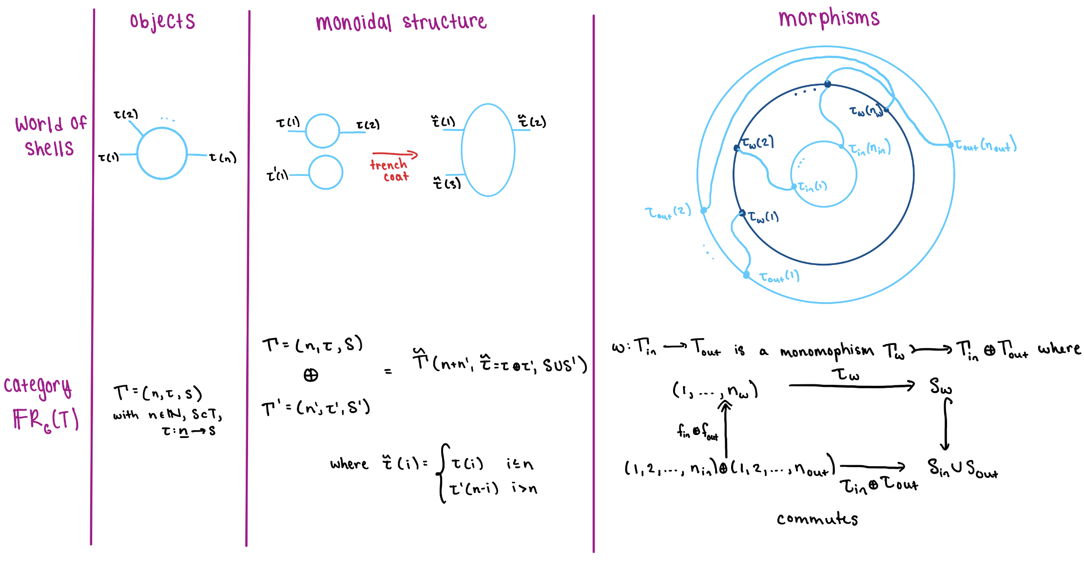
So this is the regular categorical incarnation of our pictures, and we will adorn it with a structure that mimics the behavior of the ajax functor and corresponds to the graphical actions of filling shells.
Definition: A regular calculus is a pair where is a set and is an ajax functor. A morphism of regular calculi is a pair where and is a monoidal natural transformation

that is strict in every respect.
The functor defines an ordering on the predicates that can fill each shell. Given a context , the elements of behave as predicates on and the partial ordering corresponds to entailment. For example,
Thus filling a shell with a predicate is equivalent to choosing an element of the poset . Furthermore, we are allowed to substitute one predicate for another according to the ordering of .
The next operations are trench coating and dotting off. Recall that in graphical regular logic filling the inner shells, and , of a trench coat defines a predicate for the coat, . Now that we know filling a shell corresponds to picking an element of the poset , the process of trench coating translates to: Picking an element of gives an element of . In other words we have a monotonic laxator . Monotonicity implies that commutes with entailment.
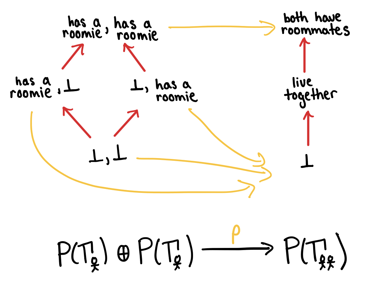
Since dotting off is a pseudo-inverse to trench coating, dotting off corresponds to an adjoint .
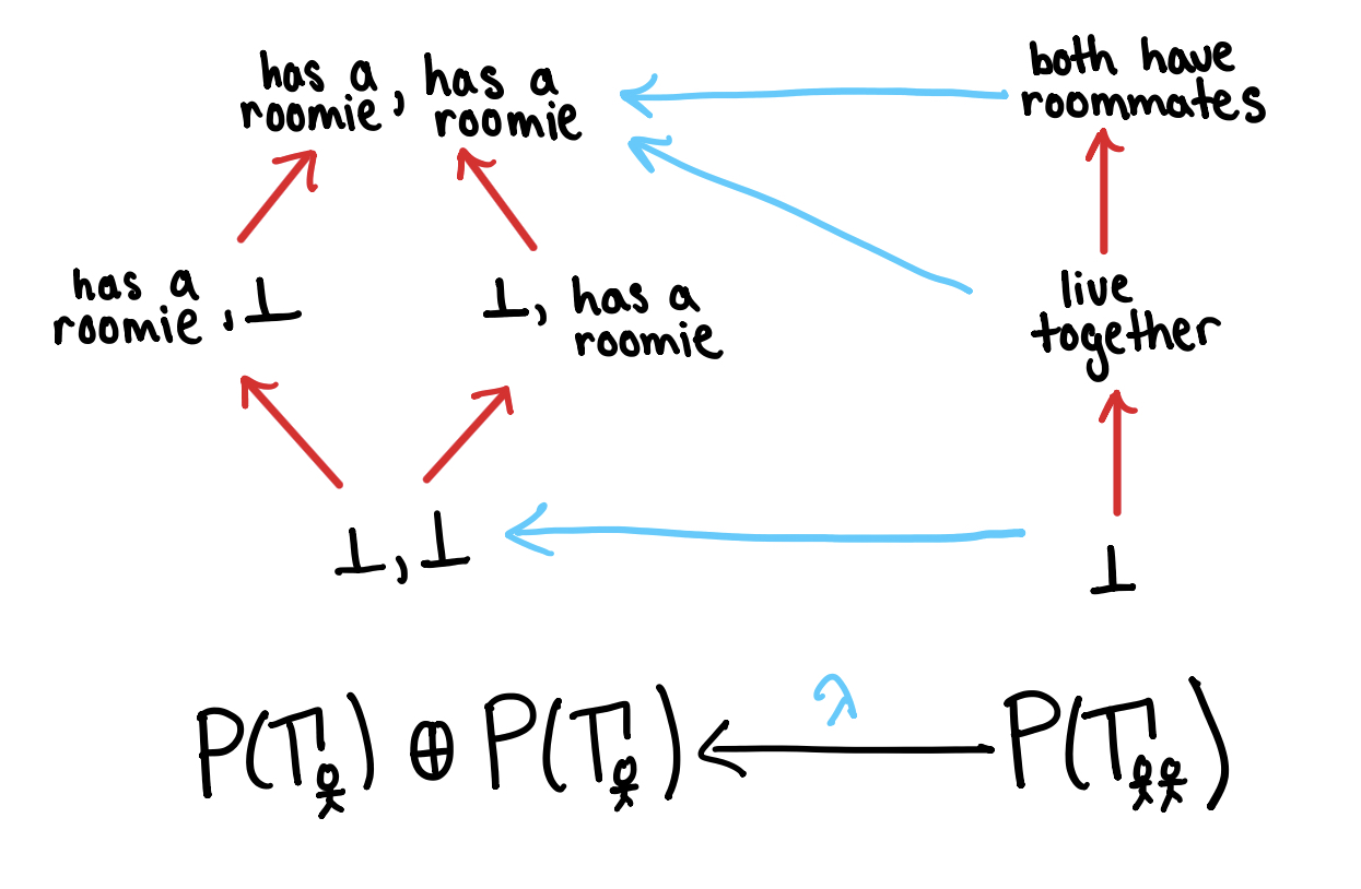
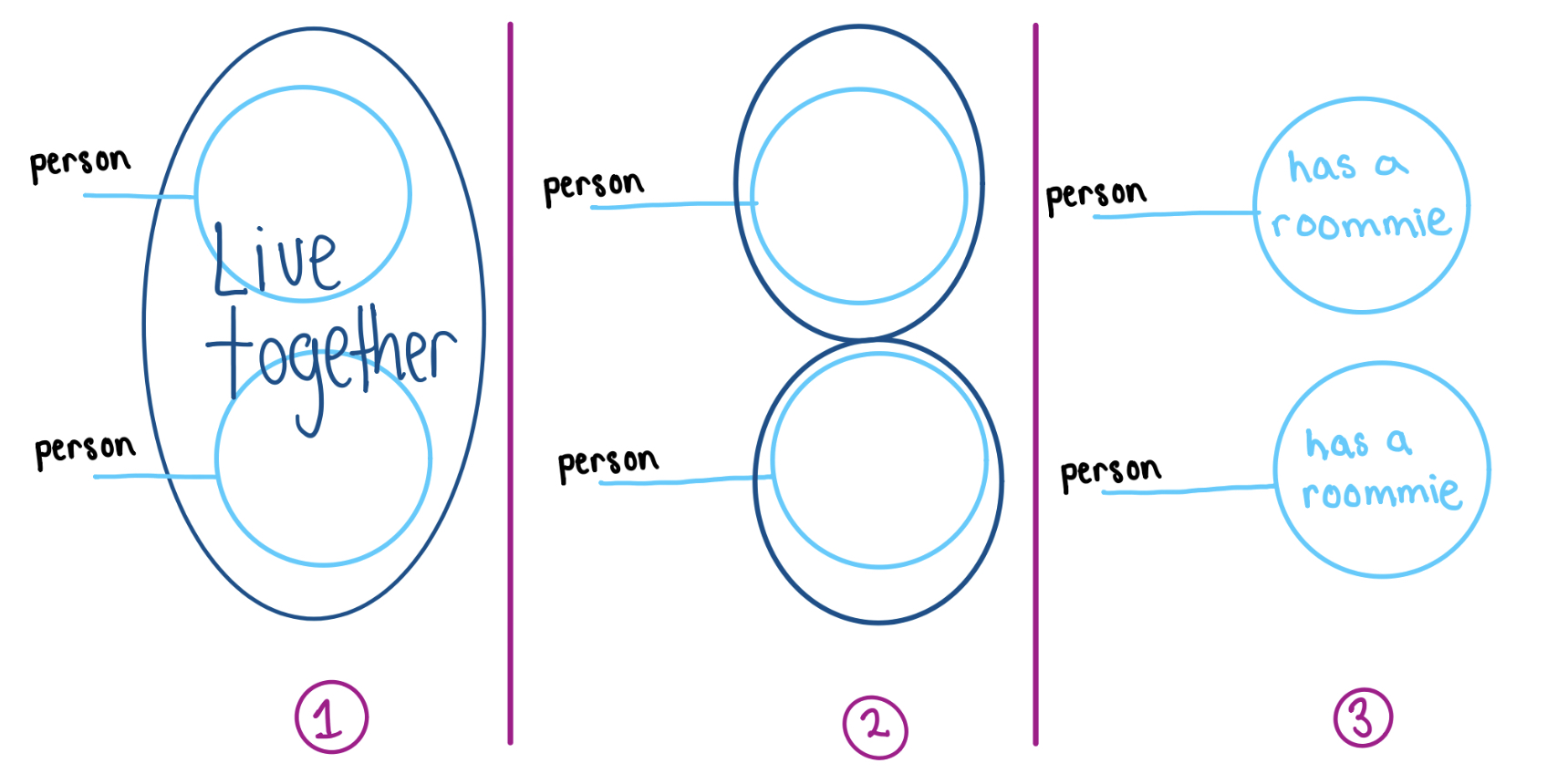
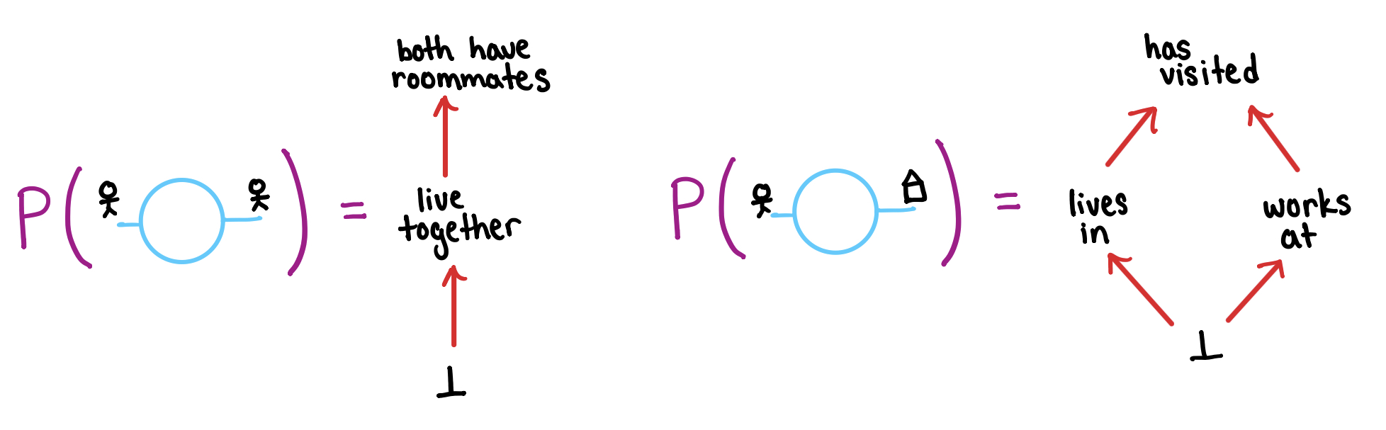
Note that dotting off and then trench coating possibly loses information. In the example below, this composition maps the predicate “live together” to the weaker predicate “both have roommates”.
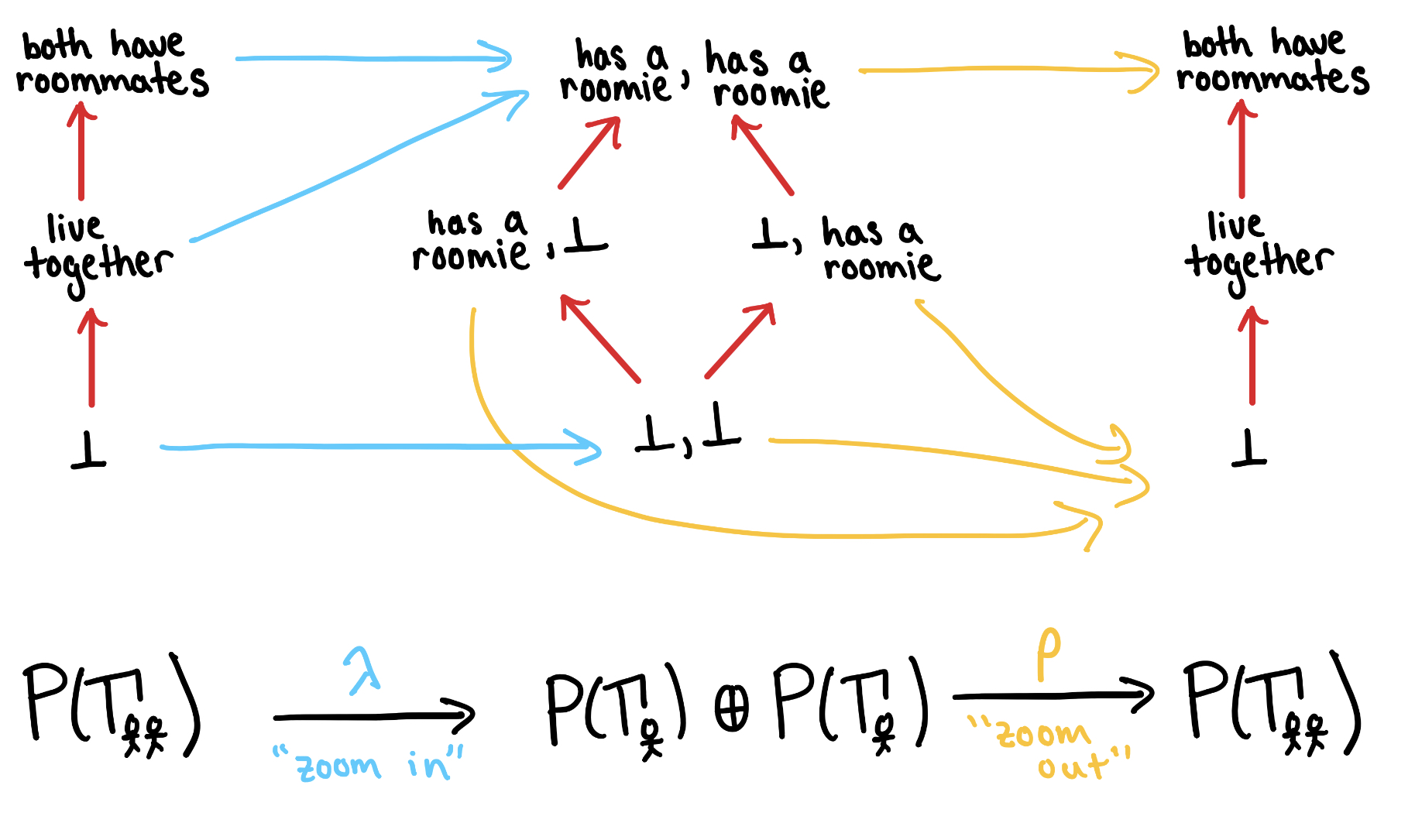
Since entails , is a right adjoint for . This is why must be ajax!
The last operation is connecting shells. Suppose we have an wiring diagram corresponding to . Like in trench coating, filling the inner shells of a wired diagram defines a predicate for the outer shell. Thus we have a map to which is given by .
If the free regular category is an incarnation of our graphical syntax, then we can think of a regular calculus as the way we stretch our definition of syntax to encompass semantics.
In particular, every regular category gives us an example of a regular calculus. If is the category of relations of a regular category, then there is an “interpretation” functor ; composing this with gives us a regular calculus whose “types” are just the objects of .
Definition: The functor is the functor sending a regular category whose category of relations is to .
The bulk of the paper is devoted to constructing a left adjoint to this functor, and proving that it is fully faithful. We’ll just give a sketch of the idea.
If we have a regular calculus , we can try and think of it as assigning to each context (object of ) its order of “subobjects”. So the objects of our “syntactic” regular category should be these “subobjects”, reified. So, for any and any , we should have an object of . This is just a fancy name for the pair , one that tells us how to think of this pair.
A relation should be a subobject of the product of the two objects represented by and , or . This should restrict nicely to and in the sense that and . Functions can now be defined as functional relations, and with no small effort one can check that this gives a regular category.
The syntactic regular category of a predicate regular calculus is equivalent to the original regular category. This means that is a reflective inclusion of regular categories into regular calculi, and justifies us using the graphical calculus, equipped with an order of “propositions” for each object varying with each signature, as a tool for reasoning about regular categories.
The reason that is not an equivalence is that changes the “types” of a graphical calculus. Perhaps if types were considered up to isomorphism in a “univalent” way, we could get an equivalence of categories; but as we move toward an equivalence between our subjective and objective logics, the less “syntactical” our subjective logic becomes.
Re: Graphical Regular Logic
Hi, When you write that I can read the diagram as “There exists a person … such that …”, do you mean “exists” in the sense of the existential quantifier (as in regular logic) or do you mean that the wire represents a free (unbound) variable?
Thanks for the article and sorry for an elementary question!