The n-Category Café

Given a lattice $L$ in $n$-dimensional Euclidean space, there’s a way to build a lattice $L^{++}$ in $(n+2)$-dimensional Minkowski spacetime. This is called the ‘over-extended’ version of $L$.

If we start with the lattice $\mathrm{E}_8$ in 8 dimensions, this process gives a lattice called $\mathrm{E}_{10}$, which plays an interesting but mysterious role in superstring theory. This shouldn’t come as a complete shock, since superstring theory lives in 10 dimensions, and it can be nicely formulated using octonions, as can the lattice $\mathrm{E}_8$.

If we start with the lattice called $\mathrm{D}_{24}$, this over-extension process gives a lattice $\mathrm{D}_{24}^{++}$. This describes the ‘cosmological billiards’ for the 3d compactification of the theory of gravity arising from bosonic string theory. Again, this shouldn’t come as a complete shock, since bosonic string theory lives in 26 dimensions.

Last time I gave a nice description of $\mathrm{E}_{10}$: it consists of $2 \times 2$ self-adjoint matrices with integral octonions as entries.

It would be nice to get a similar octonionic description of $\mathrm{D}_{24}^{++}$. But it’s actually easier to go up to 27 dimensions, because the space of $3 \times 3$ self-adjoint matrices with octonion entries is 27-dimensional. And indeed, there’s a 27-dimensional lattice waiting to be described with octonions.

You see, for any lattice $L$ in $n$-dimensional Euclidean space, there’s also a way to build a lattice $L^{+++}$ in $(n+3)$-dimensional Minkowski spacetime, called the ‘very extended’ version of $L$.

If we do this to $L = \mathrm{E}_8$ we get an 11-dimensional lattice called $\mathrm{E}_{11}$, which has mysterious connections to M-theory. But if we do it to $\mathrm{D}_{24}$ we get a 27-dimensional lattice sometimes called $\mathrm{K}_{27}$. You can read about both these lattices here:

• Peter C. West, E₁₁ and M theory.

I’ll prove that $\mathrm{E}_{11}$ has a nice description in terms of integral octonions. I’ll almost do something similar for $\mathrm{K}_{27}$, but in fact I’ll succeed for a lattice containing it, which is twice as dense.

To do these things, I’ll use the explanation of over-extended and very extended lattices given here:

• Matthias R. Gaberdiel, David I. Olive and Peter C. West, A class of Lorentzian Kac–Moody algebras.

These constructions use a 2-dimensional lattice called $\mathrm{H}$. Let’s get to know this lattice. It’s very simple.

A 2-dimensional Lorentzian lattice

Up to isometry, there’s a unique even unimodular lattice in Minkowski spacetime whenever its dimension is 2 more than a multiple of 8. The simplest of these is $\mathrm{H}$: it’s the unique even unimodular lattice in 2-dimensional Minkowski spacetime.

There are various ways to coordinatize $\mathrm{H}$. The easiest, I think, is to start with $\mathbb{R}^2$ and give it the metric $g$ with

$$g(x,x) = -2 u v$$

when $x = (u,v)$. Then, sitting in $\mathbb{R}^2$, the lattice $\mathbb{Z}^2$ is even and unimodular. So, it’s a copy of $\mathrm{H}$.

Let’s get to know it a bit. The coordinates $u$ and $v$ are called lightcone coordinates, since the $u$ and $v$ axes form the lightcone in 2d Minkowski spacetime. In other words, the vectors

$$\ell = (1,0), \quad \ell' = (0,1)$$

are lightlike, meaning

$$g(\ell,\ell) = 0 , \quad g(\ell', \ell') = 0$$

Their sum is a timelike vector

$$\tau = \ell + \ell' = (1,1)$$

since the inner product of $\tau$ with itself is negative; in fact

$$g(\tau,\tau) = -2$$

Their difference is a spacelike vector

$$\sigma = \ell - \ell' = (1,-1)$$

since the inner product of $\sigma$ with itself is positive; in fact

$$g(\sigma,\sigma) = 2$$

Since the vectors $\tau$ and $\sigma$ are orthogonal and have length $\sqrt{2}$ in the metric $g$, we get a square of area $2$ with corners

$$0, \tau, \sigma, \tau + \sigma$$

that is,

$$(0,0),\; (1,1),\; (1,-1), \;(2,0)$$

If you draw a picture, you can see by dissection that this square has twice the area of the unit cell

$$(0,0),\; (1,0), \; (0,1) , \; (1,1)$$

So, the unit cell has area 1, and the lattice is unimodular as claimed. Furthermore, every vector in the lattice has even inner product with itself, so this lattice is even.

Over-extended lattices

Given a lattice $L$ in Euclidean $\mathbb{R}^n$,

$$L^{++} = L \oplus \mathrm{H}$$

is a lattice in $(n+2)$-dimensional Minkowski spacetime, also known as $\mathbb{R}^{n+1,1}$. This lattice $L^{++}$ is called the over-extension of $L$.

A direct sum of even lattices is even. A direct sum of unimodular lattices is unimodular. Thus if $L$ is even and unimodular, so is $L^{++}$.

All this is obvious. But here are some deeper facts about even unimodular lattices. First, they only exist in $\mathbb{R}^n$ when $n$ is a multiple of 8. Second, they only exist in $\mathbb{R}^{n+1,1}$ when $n$ is a multiple of 8.

But here’s the really amazing thing. In the Euclidean case there can be lots of different even unimodular lattices in a given dimension. In 8 dimensions there’s just one, up to isometry, called $\mathrm{E}_8$. In 16 dimensions there are two. In 24 dimensions there are 24. In 32 dimensions there are at least 1,160,000,000, and the number continues to explode after that. On the other hand, in the Lorentzian case there’s just one even unimodular lattice in a given dimension, if there are any at all.

More precisely: given two even unimodular lattices in $\mathbb{R}^{n+1,1}$, they are always isomorphic to each other via an isometry: a linear transformation that preserves the metric. We then call them isometric.

Let’s look at some examples. Up to isometry, $\mathrm{E}_8$ is the only even unimodular lattice in 8-dimensional Euclidean space. We can identify it with the lattice of integral octonions, $\mathbf{O} \subseteq \mathbb{O}$, with the inner product

$$g(X,X) = 2 X X^*$$

$L^{++}$ is usually called $E_{10}$. Up to isometry, this is the unique even unimodular lattice in 10 dimensions. There are lots of ways to describe it, but last time we saw that it’s the lattice of $2 \times 2$ self-adjoint matrices with integral octonions as entries:

$$\mathfrak{h}_2(\mathbf{O}) = \left\{ \; \left( \begin{array}{cc} a & X \\ X^* & b \end{array} \right) : \; a,b \in \mathbb{Z}, \; X \in \mathbf{O} \; \right\}$$

where the metric comes from $-2$ times the determinant:

$$x = \left( \begin{array}{cc} a & X \\ X^* & b \end{array} \right) \;\; \implies \;\; g(x,x) = - \det(x) = 2 X X^* - 2 a b$$

We’ll see a fancier formula like this later on.

There are 24 even unimodular lattices in 24-dimensional Euclidean space. One of them is

$$\mathrm{E}_8 \oplus \mathrm{E}_8 \oplus \mathrm{E}_8$$

Another is $\mathrm{DD}_{24}$ the lattice of vectors in $\mathbb{R}^{24}$ where the components are either all integers or all half-integers and their sum is even. This contains the lattice $\mathrm{D}_{24}$ that I mentioned earlier. It’s twice as dense. I’ll explain it later.

If we take the over-extension of any of these even unimodular lattices in 24-dimensional Euclidean space, we get an even unimodular lattice in 26-dimensional Minkowski spacetime… and all these are isometric! The over-extension process ‘washes out the difference’ between them. In particular,

$$\mathrm{DD}_{24}^{++} \cong (\mathrm{E}_8 \oplus \mathrm{E}_8 \oplus \mathrm{E}_8)^{++}$$

This is nice because up to a scale factor, $\mathrm{E}_8$ is the lattice of integral octonions. So, there’s a description of $\mathrm{DD}_{24}^{++}$ using three integral octonions! But the story is prettier if we go up an extra dimension.

Very extended lattices

After the over-extended version $L^{++}$of a lattice $L$ in Euclidean space comes the ‘very extended’ version, called $L^{+++}$. If you ponder the paper by Gaberdiel et al, you can see this is the direct sum of the over-extension $L^{++}$ and a 1-dimensional lattice called $\mathrm{A}_1$. $\mathrm{A}_1$ is just $\mathbb{Z}$ with the metric

$$g(x,x) = 2 x^2$$

It’s even but not unimodular.

In short, the very extended version of $L$ is

$$L^{+++} = L^{++} \oplus \mathrm{A}_1 = L \oplus \mathrm{H} \oplus \mathrm{A}_1$$

If $L$ is even, so is $L^{+++}$. But if $L$ is unimodular, this will not be true of $L^{+++}$.

The very extended version of $\mathrm{E}_8$ is called $\mathrm{E}_{11}$. The very extended version of $\mathrm{D}_{24}$ is called $\mathrm{K}_{27}$. This a fascinating thing, and it would be nice to describe it using octonions. But it will be easier to work with a lattice that’s twice as dense: the very extended version of $\mathrm{DD}_{24}$.

Now it’s time to explain this ‘twice as dense’ business.

Doubling the density of D_n

The $\mathrm{D}_n$ lattice is very simple. Take an $n$-dimensional checkerboard with alternating red and black hypercubes. Put a dot in the middle of each black hypercube. That’s the $\mathrm{D}_n$ lattice!

More precisely, the $\mathrm{D}_n$ lattice consists of all $n$-tuples of integers that sum to an even integer. Requiring that they sum to an even integer picks out the center of every other hypercube in our checkerboard.

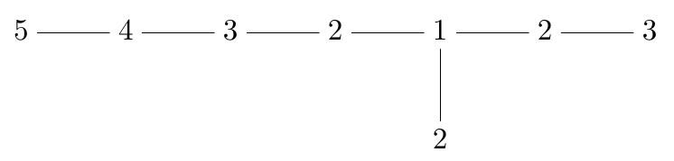
Here’s a basis of vectors for the $\mathrm{D}_4$ lattice:

$$\begin{array}{cccc} (-1, & -1, & 0, & 0) \\ (1, & -1, & 0, & 0 ) \\ (0, & 1, & -1 & 0 ) \\ (0, & 0, & 1, & -1) \end{array}$$

The same pattern works in any dimension: the first vector has two $-1$s followed by a bunch of zeros, but the rest of the vectors are all just shifted versions of the second. I’ve chosen them to be simple roots for $\mathrm{D}_n$, but that’s not so important now.

What really matters is this. The dot product of any basis vector with itself is even, and the dot product of any two different ones is an integer. Thus, the lattice they generate, the $\mathrm{D}_n$ lattice, is even: the dot product of any vector with itself is even.

Also, the determinant of the matrix formed by our basis vectors:

$$\left( \begin{array}{rrrr} -1 & -1 & 0 & 0 \\ 1 & -1 & 0 & 0 \\ 0 & 1 & -1 & 0 \\ 0 & 0 & 1 & -1 \end{array} \right)$$

is 2. In any dimension, this sort of determinant gives $\pm 2$. So, the volume of the unit cell in $\mathrm{D}_n$ lattice is always 2. So, it’s not unimodular.

To get something unimodular, we can double the density by taking the union of $\mathrm{D}_n$ and a copy of $\mathrm{D}_n$ translated by the vector

$$\left(\frac{1}{2}, \dots, \frac{1}{2} \right)$$

Let’s call this union $\mathrm{DD}_n$. A lot of people call it $\mathrm{D}_n^+$, but we’re using plus signs for too many other things already. I’m calling it $\mathrm{D}_n$ because it’s doubly dense, and also because it’s the union of two shifted copies of $\mathrm{D}_n$.

$\mathrm{DD}_3$ is the way carbon atoms are arranged in a diamond!

This pattern is called the diamond cubic. It’s beautiful, but it’s not a lattice in the mathematical sense. $\mathrm{DD}_n$ is a lattice only when $n$ is even. Here’s the story:

• In any dimension, the volume of the Voronoi cells of $\mathrm{DD}_n$ is 1, so we can say it’s unimodular.
• In even dimensions, and only those, $\mathrm{DD}_n$ is lattice. After all, only then does the sum of $(\frac{1}{2}, \dots, \frac{1}{2})$ with itself again lie in $\mathrm{DD}_n$.
• In dimensions that are multiples of 4, and only those, $\mathrm{DD}_n$ is an integral lattice, meaning that the dot product of any two vectors in the lattice is an integer. After all, only then is the inner product of $(\frac{1}{2}, \dots, \frac{1}{2})$ with itself an integer.
• In dimensions that are multiples of 8, and only those, $\mathrm{DD}_n$ is an even lattice, meaning that the dot product of any vector with itself is even. After all, only then is the inner product of $(\frac{1}{2}, \dots, \frac{1}{2})$ even.

As I mentioned before, even unimodular lattices are possible in Euclidean space only when the dimension is a multiple of 8. $\mathrm{DD}_8$ is none other than our friend $\mathrm{E}_8$! But what we really need now is $\mathrm{DD}_{24}$, since it’s an even unimodular lattice in 24 dimensions. I’d like to have a nice octonionic description of

$$\mathrm{K}_{27} = \mathrm{D}_{24}^{+++}$$

but I’ll actually get one for

$$\mathrm{DD}_{24}^{+++}$$

which is twice as dense. We could use this to get an octonionc description of $\mathrm{K}_{27}$, but I won’t do that.

Lattices in the exceptional Jordan algebra

Now we are ready to have some fun!

Let $\mathfrak{h}_3(\mathbb{O})$ be the space of $3 \times 3$ self-adjoint octonionic matrices. It’s 27-dimensional since a typical element looks like

$$x = \left( \begin{array}{ccc} a & X & Y \\ X^* & b & Z \\ Y^* & Z^* & c \end{array} \right)$$

where $a,b,c \in \mathbb{R}, X,Y,Z \in \mathbb{O}$. It’s called the exceptional Jordan algebra. We don’t need to know about Jordan algebras now, but this concept encapsulates the fact that if $x \in \mathfrak{h}_3(\mathbb{O})$, so is $x^2$.

There’s a 2-parameter family of metrics on the exceptional Jordan algebra that are invariant under all Jordan algebra automorphisms. They have

$$g(x,x) = \alpha \tr(x^2) + \beta \tr(x)^2$$

for $\alpha, \beta \in \mathbb{R}$ with $\alpha \ne 0$. Some are Euclidean and some are Lorentzian.

Sitting inside the exceptional Jordan algebra is the lattice of $3 \times 3$ self-adjoint matrices with integral octonions as entries:

$$\mathfrak{h}_3(\mathbf{O}) = \left\{ \; \left( \begin{array}{ccc} a & X & Y \\ X^* & b & Z \\ Y^* & Z^* & c \end{array} \right) :\; a,b,c \in \mathbb{Z}, \; X,Y,Z \in \mathbf{O} \; \right\}$$

And here’s the cool part:

Theorem. There is a Lorentzian inner product $g$ on the exceptional Jordan algebra that is invariant under all automorphisms and makes the lattice $\mathfrak{h}_3(\mathbf{O})$ isometric to $\mathrm{DD}_{24}^{+++}$.

Proof. We will prove that the metric

$$g(x,x) = \tr(x^2) - \tr(x)^2$$

obeys all the conditions of this theorem. From what I’ve already said, it is invariant under all Jordan algebra automorphisms. The challenge is to show that it makes $\mathfrak{h}_3(\mathbf{O})$ isometric to $\mathrm{DD}_{24}^{+++}$. But instead of $\mathrm{DD}_{24}^{+++}$, we can work with $(\mathrm{E}_8 \oplus \mathrm{E}_8 \oplus \mathrm{E}_8)^{+++}$, since we have seen that

$$\mathrm{DD}_{24}^{+++} \cong (\mathrm{E}_8 \oplus \mathrm{E}_8 \oplus \mathrm{E}_8)^{+++}$$

Let us examine the metric $g$ in more detail. Take any element $x \in \mathfrak{h}_3(\mathbf{O})$:

$$x = \left( \begin{array}{ccc} a & X & Y \\ X^* & b & Z \\ Y^* & Z^* & c \end{array} \right)$$

where $a,b,c \in \mathbb{R}, X,Y,Z \in \mathbb{O}$. Then

$$tr(x^2) = a^2 + b^2 + c^2 + 2(X X^* + Y Y^* + Z Z^*)$$

while

$$tr(x)^2 = (a + b + c)^2$$

Thus

$$\begin{array}{ccl} g(x,x) &=& tr(x^2) - tr(x)^2 \\ &=& 2(X X^* + Y Y^* + Z Z^*) - 2(a b + b c + c a) \end{array}$$

It follows that with this metric, the diagonal matrices are orthogonal to the off-diagonal matrices. An off-diagonal matrix $x \in \mathfrak{h}_3(\mathbf{O})$ is a triple $(X,Y,Z) \in \mathbf{O}^3$, and has

$$g(x,x) = 2(X X^* + Y Y^* + Z Z^*)$$

Thanks to the factor of 2, this metric makes the lattice of these off-diagonal matrices isometric to $\mathrm{E}_8 \oplus \mathrm{E}_8 \oplus \mathrm{E}_8$. Since

$$(\mathrm{E}_8 \oplus \mathrm{E}_8 \oplus \mathrm{E}_8)^{+++} = \mathrm{E}_8 \oplus \mathrm{E}_8 \oplus \mathrm{E}_8 \oplus \mathrm{H} \oplus \mathrm{A}_1$$

it thus suffices to show that the 3-dimensional Lorentzian lattice of diagonal matrices in $\mathfrak{h}_3(\mathbf{O})$ is isometric to

$$\mathrm{H} \oplus \mathrm{A}_1$$

A diagonal matrix $x \in \mathfrak{h}_3(\mathbf{O})$ is a triple $(a,b,c) \in \mathbb{Z}^3$, and on these triples the inner product $g$ is given by

$$g(x,x) = -2(a b + b c + c a)$$

If we restrict attention to triples of the form $x = (a,b,0)$, we get a 2-dimensional Lorentzian lattice: a copy of $\mathbb{Z}^2$ with inner product

$$g(x,x) = -2a b$$

This is just $\mathrm{H}$.

We can use this to show that the lattice of all triples $(a,b,c) \in \mathbb{Z}^3$, with the inner product $g$, is isometric to $\mathrm{H} \oplus \mathrm{A}_1$.

Remember, $\mathrm{A}_1$ is a 1-dimensional lattice generated by a spacelike vector whose norm squared is 2. So, it suffices to show that the lattice $\mathbb{Z}^3$ is generated by vectors of the form $(a,b,0)$ together with a spacelike vector of norm squared 2 that is orthogonal to all those of the form $(a,b,0)$.

To do this, we need to describe the inner product $g$ on $\mathbb{Z}^3$ more explicitly. For this, we can use polarization identity

$$g(x,x') = \frac{1}{2}( g(x+x',x+x') - g(x,x) - g(x',x'))$$

Remember, if $x = (a,b,c)$ we have

$$g(x,x) = -2(a b + b c + c a)$$

So, if we also have $x' = (a',b',c')$, the polarization identity gives

$$g(x,x') = -(a b'+a' b) - (b c'+ b c') - (c a' + c'a)$$

We are looking for a spacelike vector $x' = (a',b',c')$ that is orthogonal to all those of the form $x = (a,b,0)$. For this, it is necessary and sufficient to have

$$0 = g((1,0,0),(a',b',c')) = - b' - c'$$

and

$$0 = g((0,1,0), (a',b',c')) = - a' - c'$$

An example is $x' = (1,1,-1)$. This has

$$g(x',x') = -2(1 - 1 - 1) = 2$$

so it is spacelike, as desired. Even better, it has norm squared two. And even better, this vector $x'$, along with those of the form $(a,b,0)$, generates the lattice $\mathbb{Z}^3$.

So we have shown what we needed: the lattice of all triples $(a,b,c) \in \mathbb{Z}^3$ is generated by those of the form $(a,b,0)$ together with a spacelike vector with norm squared 2 that is orthogonal to all those of the form $(a,b,0)$. $\blacksquare$

This theorem has three nice spinoffs:

Corollary 1. With the same Lorentzian inner product $g$ on the exceptional Jordan algebra, the lattice $\mathrm{DD}_{24}^{++}$ is isometric to the sublattice of $\mathfrak{h}_3(\mathbf{O})$ where a fixed diagonal entry is set equal to zero, e.g.:

$$\left\{ \; \left( \begin{array}{ccc} a & X & Y \\ X^* & b & Z \\ Y^* & Z^* & 0 \end{array} \right) : \; a,b \in \mathbb{Z}, \; X,Y,Z \in \mathbf{O} \; \right\}$$

Proof. Use the fact that with the metric $g$, the diagonal matrices

$$\left\{ \; \left( \begin{array}{ccc} a & 0 & 0 \\ 0 & b & 0 \\ 0 & 0 & 0 \end{array} \right) : \; a,b \in \mathbb{Z} \; \right\}$$

form a copy of $\mathrm{H}$, so the matrices above form a copy of

$$\mathrm{E}_8 \oplus \mathrm{E}_8 \oplus \mathrm{E}_8 \oplus \mathrm{H} \cong (\mathrm{E}_8 \oplus \mathrm{E}_8 \oplus \mathrm{E}_8)^{++} \cong \mathrm{DD}_{24}^{++} \qquad \qquad \qquad \blacksquare$$

Corollary 2. With the same Lorentzian inner product $g$ on the exceptional Jordan algebra, the lattice $\mathrm{E}_{11} = E_8^{+++}$ is isometric to the sublattice of $\mathfrak{h}_3(\mathbf{O})$ where two fixed off-diagonal entries are set equal to zero, e.g.:

$$\left\{ \; \left( \begin{array}{ccc} a & X & 0 \\ X^* & b & 0 \\ 0 & 0 & c \end{array} \right) : \; a,b,c \in \mathbb{Z}, \; X\in \mathbf{O} \; \right\}$$

Proof. Use the fact that with the metric $g$, the diagonal matrices

$$\left\{ \; \left( \begin{array}{ccc} a & 0 & 0 \\ 0 & b & 0 \\ 0 & 0 & c \end{array} \right) : \; a,b \in \mathbb{Z} \; \right\}$$

form a copy of $\mathrm{H} \oplus \mathrm{A}_1$, so the matrices above form a copy of

$$\mathrm{E}_8 \oplus \mathrm{H} \oplus \mathrm{A}_1 \cong \mathrm{E}_8^{+++} \qquad \qquad \qquad \blacksquare$$

Corollary 3. With the same Lorentzian inner product $g$ on the exceptional Jordan algebra, the lattice $\mathrm{E}_{10} = \mathrm{E}_8^{++}$ is isometric to the sublattice of $\mathfrak{h}_3(\mathbf{O})$ where two fixed off-diagonal entries and one diagonal entry are set equal to zero, e.g.:

$$\left\{ \; \left( \begin{array}{ccc} a & X & 0 \\ X^* & b & 0 \\ 0 & 0 & 0 \end{array} \right) : \; a,b,c \in \mathbb{Z}, \; X\in \mathbf{O} \; \right\}$$

Proof. Use the previous corollary; this is the obvious copy of $\mathrm{E}_8^{++} \cong \mathrm{E}_8 \oplus \mathrm{H}$ inside $\mathrm{E}_8^{+++} \cong \mathrm{E}_8 \oplus \mathrm{H} \oplus \mathrm{A}_1$. $\blacksquare$