The n-Category Café

Wow! Exquisite as those pictures by Christensen and Derbyshire are, what really gets me is that this is such an obvious thing to do, yet apparently no one had thought to do it before. (Or had they?)

It reminds me of something I read about the resurgence of interest in complex dynamics, in the late 1970s. (If I understand correctly, the field had been largely dormant since about 1920, when Fatou and Julia did their pioneering work.) A bunch of people, including Brooks, Matelski, Douady, Hubbard and Mandelbrot, began to study the iteration of quadratic maps, with the aid of the emerging computer technology.

Douady was working in Paris, close to the IHES. It must have been an amazing place and time. Deligne had solved the Weil conjectures not so long ago. And Douady… Douady was studying quadratic equations. There’s some interview with or about him, which I can’t find now, where he recalls someone asking “These quadratics — do you really hope to find anything new?”

And while I’m recalling anecdotes, I can’t resist adding this one, from Milnor’s book Dynamics in One Complex Variable.

Mandelbrot made quite good computer pictures [of the Mandelbrot set, about 1980], which seemed to show a number of isolated “islands”. Therefore, he conjectured that [the Mandelbrot set] has many distinct connected components. (The editors of the journal thought that his islands were specks of dirt, and carefully removed them from the pictures.)

Hi John,

so, basically your friend discovered the first fractal that was not generated by any kind of iterative process! WOW!

3-categories for the working mathematician

404 Not Found

I can't figure out what the URI should really be.

A long knot is a curve in R³ that goes on forever and is a vertical straight line outside some compact set.

In other words, a long knot is a 1-strand tangle.

These are more like the knots in ordinary life; it's always a little disconcerting to tell people that mathematicians' knots are closed up end to end.

So, where’s the almond blot? (I’m not being entirely facetious; it’s been known to turn up between attracting basins for various Newton-Raphson itterations, of all places.)

I also can’t help noticing that, if $P(x),Q(x)$ have $\pm 1$ coefficients, and $Q$ is of degree $d-1$, then $Q(x) P(x^d)$ also has coefficients $\pm 1$. That would be more than enough to describe the cloudiness of the picture near the unit circle: it’ll have all the $d^{th}$ roots of simpler roots — so a copy of the larger pattern repeating $d$ times, roughly a factor of $d$ closer to the circle — although with the polynomials here, $d$ or the degree of $P$ will be small, so it’s not a good model for “small” pictures like this. In a correlative direction, any guess about how many of these polynomials are irreducible?

The pictures on week285 are all low-resolution or partial versions of Sam Derbyshire’s original image. The original is available as a 90-megabyte file here.

Some of my Windows software is unable to display such a large file — it claims the file is corrupted. But irfanview can handle it. Slow, though!

I can think of a true first-order sentence involving quandles that doesn’t seem provable from the axioms (indeed, I don’t think it’s expressible as an equation), which is that, for any g, h in the quandle, there’s another element of the quandle, call it “gh,” such that

g > (h > k) = gh > k

for all k in the quandle. This is obvious if you write it out in the underlying group.

But gh (as an element of the group) can’t necessarily be written in terms of quandle elements and operations, since it might lie in a different conjugacy class than both g and h.

Of course this can’t directly be turned into an equation, but it seems like the major stumbling block in trying to prove that the quandle relations you give are complete.

I’m a bit out of my league here, but a fractal can be constructed by taking an initial set of points and applying an affine transformation. It’s how IFS fractals are made anyway I think.

It would then seem that we can do an affine transformation of a set of solutions to arrive at new solutions. But why the particular affine transformation producing this fractal?

Remembering that the roots of any polynomial may be written in terms of multivariate hypergeometric functions it seems to me that doi:10.1016/j.bulsci.2006.12.004 among others are touching on this topic.

A few people have used the word “fractal” in connection with these pictures. This makes me rather puzzled.

On the one hand, the spaces portrayed are finite. John wrote, in TWF:

Let’s define the set $C(d,n)$ to be the set of all roots of all polynomials of degree [at most] $d$ with integer coefficients ranging from $-n$ to $n$.

These spaces $C(d, n)$ are finite. All the pictures in TWF are of $C(d, n)$ (or a subset thereof) for some choice of $d$ and $n$; so all the pictures are of finite spaces. To be clear: the pictures aren’t finite approximations to infinite spaces, as many pictures of fractals are. The spaces being portrayed really are finite.

Now, from most points of view finite spaces are very boring. In particular, they have dimension $0$ in just about any sense of “dimension” you like. One characteristic property of fractals (a word for which there’s no agreed definition) is that the Hausdorff dimension is greater than the topological dimension. But that’s not the case here. Another general feature is that as you zoom in, you keep seeing more detail. Again, that’s not the case here.

So, it seems hard to say that these spaces are in any sense fractals.

On the other hand, look at them! They have a clear resemblance to all the things we call fractals. So, are these spaces $C(d, n)$ approximations to some fractal space? John wrote:

Clearly $C(d,n)$ gets bigger as we make either $d$ or $n$ bigger. It becomes dense in the complex plane as $n \to \infty$, as long as $d \geq 1$ [should be $d \geq 2$?]. We get all the rational complex numbers if we fix $d \geq 1$ [2?] and let $n \to \infty$, and all the algebraic complex numbers if let both $d,n \to \infty$.

But what happens if we fix $n$ and let $d \to \infty$? Write $$C(\infty, n) = \bigcup_{d = 0}^\infty C(d, n).$$ E.g. $C(\infty, 1)$ is the set of all $z \in \mathbb{C}$ satisfying some equation such as $$z^3 + z^5 = z^4 + z^7 + z^{11}.$$ I can’t figure out anything at all about this set. Is it dense in $\mathbb{C}$? Bounded? Unbounded? Is it, in fact, some fractal space of which the finite spaces $C(d, n)$ are approximations?

John mentioned Odlyzko and Poonen’s result on polynomials with coefficients in $\{0, 1\}$ (as opposed to $\{-1, 0, 1\}$, the example just mentioned). There, you don’t get anything like all of $\mathbb{C}$; in fact, all the roots lie in a certain annulus. But that asymmetric constraint on the coefficients strikes me as changing the character of the problem.

Let’s try to make some rigorous definitions. Let $R(n)$ be the measure on $\mathbb{CP}^1$ which has weight $1/(n 3^{n+1})$ on each of the points in $C(1,n)$. (There are $3^{n+1}$ degree $n$ polynomials whose coefficients are in $\{ -1, 0,1 \}$; hence $n 3^{n+1}$ roots.)

What is the support of the limit measure? Can we find some easy sets in the complement? Can we show that the Hausdorff dimension is fractional?

The sequence above shows subsets of the Derbyshire set of order 16 (i.e. roots of polynomials of order 16 whose coefficients belong to $\{-1,1\}$), with each frame coming from polynomials with a particular sum of coefficients (or equivalently, a particular number of coefficients equal to $1$ rather than $-1$).

It’s interesting that at least some of the “fractal” structure seems to be present within the largest of these subsets, as opposed to needing all of the subsets combined to make it apparent. So I guess something interesting must arise solely from permuting the coefficients, at least when there are roughly equal numbers of $1$s and $-1$s.

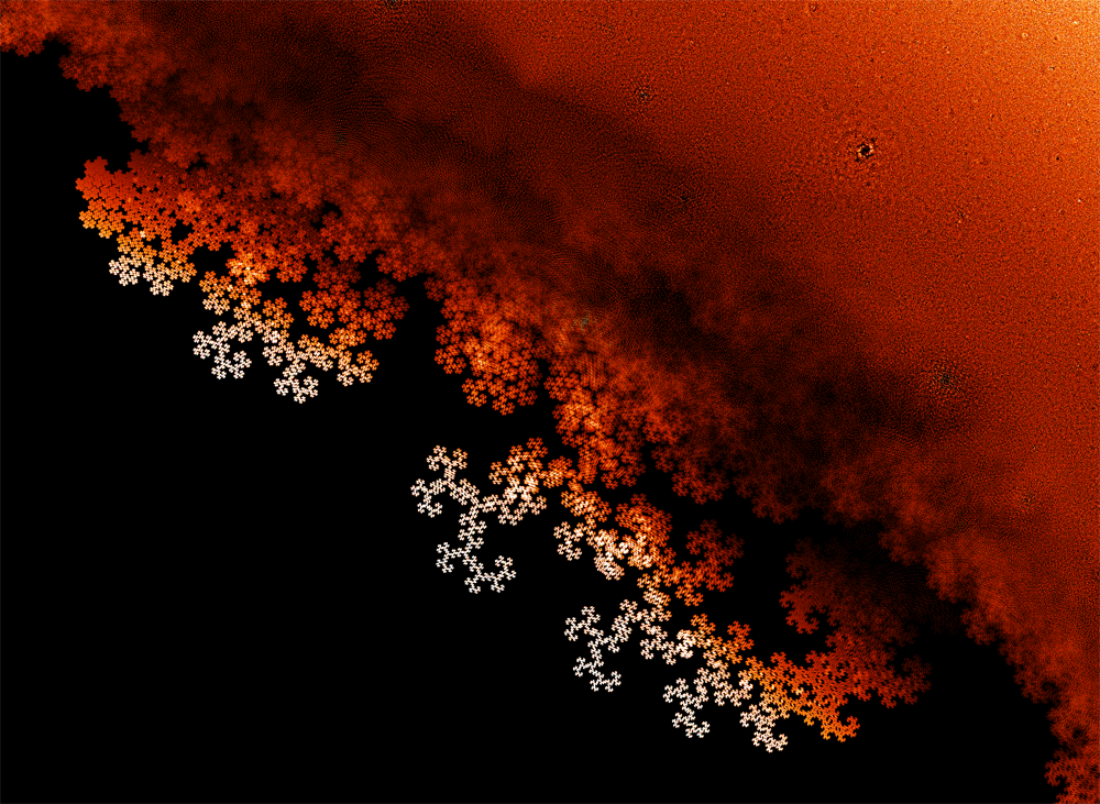
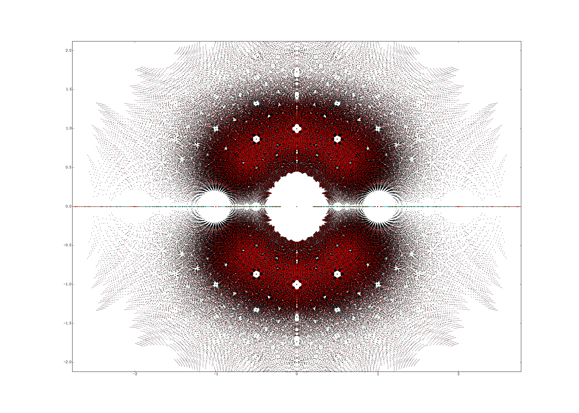
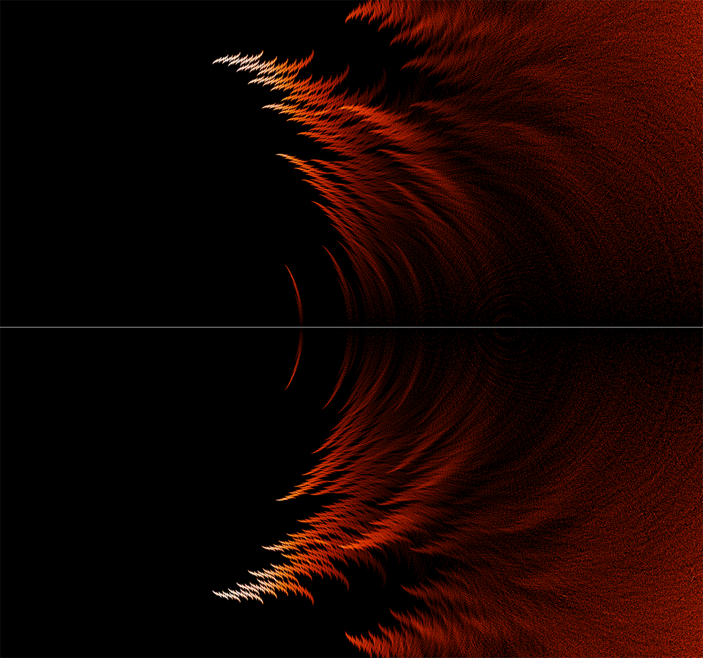
Above are the roots of some polynomials with 8 coefficients of 1 and 9 of -1:

$$z^{16}+z^{15}+z^{14}+z^{13}+z^{12}+z^{11}+z^{10}+z^9-z^8-z^7-z^6-z^5-z^4-z^3-z^2-z-1$$

$$z^{16}+z^{15}+z^{14}+z^{13}+z^{12}+z^{11}+z^{10}-z^9+z^8-z^7-z^6-z^5-z^4-z^3-z^2-z-1$$

$$z^{16}+z^{15}+z^{14}+z^{13}+z^{12}+z^{11}+z^{10}-z^9-z^8+z^7-z^6-z^5-z^4-z^3-z^2-z-1$$

$$z^{16}+z^{15}+z^{14}+z^{13}+z^{12}+z^{11}+z^{10}-z^9-z^8-z^7+z^6-z^5-z^4-z^3-z^2-z-1$$

$$z^{16}+z^{15}+z^{14}+z^{13}+z^{12}+z^{11}+z^{10}-z^9-z^8-z^7-z^6+z^5-z^4-z^3-z^2-z-1$$

$$z^{16}+z^{15}+z^{14}+z^{13}+z^{12}+z^{11}+z^{10}-z^9-z^8-z^7-z^6-z^5+z^4-z^3-z^2-z-1$$

$$z^{16}+z^{15}+z^{14}+z^{13}+z^{12}+z^{11}+z^{10}-z^9-z^8-z^7-z^6-z^5-z^4+z^3-z^2-z-1$$

$$z^{16}+z^{15}+z^{14}+z^{13}+z^{12}+z^{11}+z^{10}-z^9-z^8-z^7-z^6-z^5-z^4-z^3+z^2-z-1$$

$$z^{16}+z^{15}+z^{14}+z^{13}+z^{12}+z^{11}+z^{10}-z^9-z^8-z^7-z^6-z^5-z^4-z^3-z^2+z-1$$

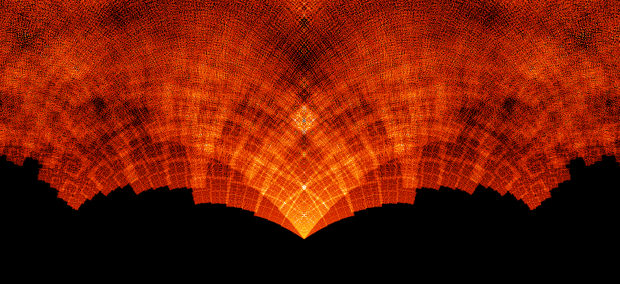
Above are the roots of some polynomials with 9 coefficients of 1 and 8 of -1:

$$z^{16}+z^{15}+z^{14}+z^{13}+z^{12}+z^{11}+z^{10}+z^9+z^8-z^7-z^6-z^5-z^4-z^3-z^2-z-1$$

$$z^{16}+z^{15}+z^{14}+z^{13}+z^{12}+z^{11}+z^{10}+z^9-z^8+z^7-z^6-z^5-z^4-z^3-z^2-z-1$$

$$z^{16}+z^{15}+z^{14}+z^{13}+z^{12}+z^{11}+z^{10}+z^9-z^8-z^7+z^6-z^5-z^4-z^3-z^2-z-1$$

$$z^{16}+z^{15}+z^{14}+z^{13}+z^{12}+z^{11}+z^{10}+z^9-z^8-z^7-z^6+z^5-z^4-z^3-z^2-z-1$$

$$z^{16}+z^{15}+z^{14}+z^{13}+z^{12}+z^{11}+z^{10}+z^9-z^8-z^7-z^6-z^5+z^4-z^3-z^2-z-1$$

$$z^{16}+z^{15}+z^{14}+z^{13}+z^{12}+z^{11}+z^{10}+z^9-z^8-z^7-z^6-z^5-z^4+z^3-z^2-z-1$$

$$z^{16}+z^{15}+z^{14}+z^{13}+z^{12}+z^{11}+z^{10}+z^9-z^8-z^7-z^6-z^5-z^4-z^3+z^2-z-1$$

$$z^{16}+z^{15}+z^{14}+z^{13}+z^{12}+z^{11}+z^{10}+z^9-z^8-z^7-z^6-z^5-z^4-z^3-z^2+z-1$$

$$z^{16}+z^{15}+z^{14}+z^{13}+z^{12}+z^{11}+z^{10}+z^9-z^8-z^7-z^6-z^5-z^4-z^3-z^2-z+1$$

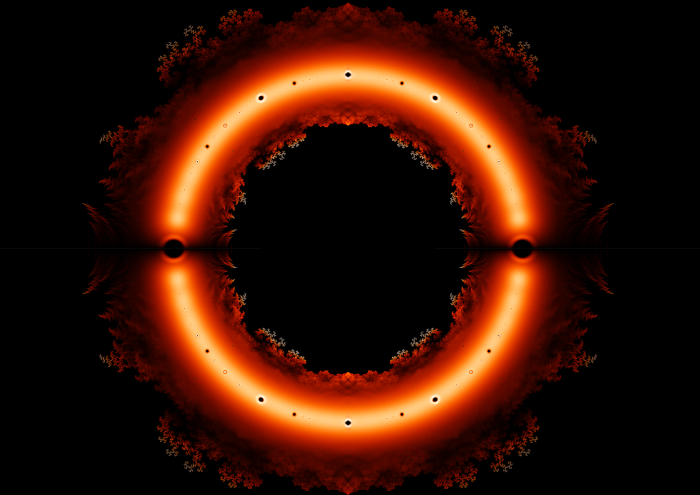
Above are the roots of some polynomials with 10 coefficients of 1 and 7 of -1:

$$z^{16}+z^{15}+z^{14}+z^{13}+z^{12}+z^{11}+z^{10}+z^9+z^8+z^7-z^6-z^5-z^4-z^3-z^2-z-1$$

$$z^{16}+z^{15}+z^{14}+z^{13}+z^{12}+z^{11}+z^{10}+z^9+z^8-z^7+z^6-z^5-z^4-z^3-z^2-z-1$$

$$z^{16}+z^{15}+z^{14}+z^{13}+z^{12}+z^{11}+z^{10}+z^9+z^8-z^7-z^6+z^5-z^4-z^3-z^2-z-1$$

$$z^{16}+z^{15}+z^{14}+z^{13}+z^{12}+z^{11}+z^{10}+z^9+z^8-z^7-z^6-z^5+z^4-z^3-z^2-z-1$$

$$z^{16}+z^{15}+z^{14}+z^{13}+z^{12}+z^{11}+z^{10}+z^9+z^8-z^7-z^6-z^5-z^4+z^3-z^2-z-1$$

$$z^{16}+z^{15}+z^{14}+z^{13}+z^{12}+z^{11}+z^{10}+z^9+z^8-z^7-z^6-z^5-z^4-z^3+z^2-z-1$$

$$z^{16}+z^{15}+z^{14}+z^{13}+z^{12}+z^{11}+z^{10}+z^9+z^8-z^7-z^6-z^5-z^4-z^3-z^2+z-1$$

$$z^{16}+z^{15}+z^{14}+z^{13}+z^{12}+z^{11}+z^{10}+z^9+z^8-z^7-z^6-z^5-z^4-z^3-z^2-z+1$$

$$z^{16}+z^{15}+z^{14}+z^{13}+z^{12}+z^{11}+z^{10}+z^9-z^8+z^7+z^6-z^5-z^4-z^3-z^2-z-1$$

The general effect seems to be that as you shift the coefficient that gets the plus sign you can move the roots around various curves, but I can’t see any simple formula for what’s going on here.

One more example of a tight spiral of roots as we shift a sign along the coefficients. These five roots are from the polynomials:

$$z^{16}-z^{15}+z^{14}+z^{13}+z^{12}-z^{11}-z^{10}+z^9+z^8+z^7+z^6+z^5-z^4-z^3-z^2-z+1$$

$$z^{16}-z^{15}+z^{14}+z^{13}+z^{12}-z^{11}-z^{10}+z^9+z^8+z^7+z^6+z^5-z^4-z^3-z^2+z-1$$

$$z^{16}-z^{15}+z^{14}+z^{13}+z^{12}-z^{11}-z^{10}+z^9+z^8+z^7+z^6+z^5-z^4-z^3+z^2-z-1$$

$$z^{16}-z^{15}+z^{14}+z^{13}+z^{12}-z^{11}-z^{10}+z^9+z^8+z^7+z^6+z^5-z^4+z^3-z^2-z-1$$

$$z^{16}-z^{15}+z^{14}+z^{13}+z^{12}-z^{11}-z^{10}+z^9+z^8+z^7+z^6+z^5+z^4-z^3-z^2-z-1$$

Here’s a very rough explanation as to why we should expect “fractal” spirals to appear in these root sets.

Suppose we have a polynomial in our set, $R(z)$, with a root at $z=r$. And suppose there’s a family of other polynomials in our set, which are all related to $R(z)$ by:

$$P_n(z)=R(z)+a z^n$$

where $a$ is a constant. A Taylor expansion about $z=r$ gives:

$$P_n(r+w)\approx a r^n + (n a r^{n-1} + R'(r))w$$

So (in so far as the Taylor expansion is useful for approximating roots of $P_n(z)$ near $r$), we can expect roots $r_n$ of approximately:

$$r_n\approx r - \frac{a r^n}{n a r^{n-1} + R'(r)}$$

If $R'(r)$ dominates $n a r^{n-1}$, we’d expect a spiral pattern centred on the original root $r$:

$$r_n\approx r - b r^n$$

where $b=\frac{a}{R'(r)}$.

Of course this is all pretty crude and hand-wavy, but qualitatively it says: expect sometimes to see roots occur in spirals around other roots, at scales that can be expected to shrink as $R'(r)$ gets large.

For curiosity, I had sage plot the least absolute value of Derbyshire’s polynomials up to degree 7, (if I’ve counted right); and you can sort-of see some of the dragon shapes starting to shape-up around the edges:

otherwise, it’s not a great picture. I asked for 300x300 resolution, but I don’t believe this shows that much.

Incidentally, does anyone know how to ask sage to just plot colours, or must I get them indirectly from a 3d-plot?

Here’s a heuristic way of understanding why the set of roots of the Littlewood polynomials that lie near $z$ resembles the set of images of $z$ under the same Littlewood polynomials.

The image of $z$ under all the Littlewood polynomials is the same as iterating with every possible composition of the maps $f_{z,+}(x)=1+z x$ and $f_{z,-}(x)=1-z x$, applied to a “seed point” of $0$. If we get a nice fractal from that Iterated Function System, then if we zoom in close to the origin we should see something qualitatively the same.

In the picture above, $z$ is mapped to a set of points near $0$ by some subset of the Littlewood polynomials. This image is just a subset of the image of $z$ under all the polynomials, but because the complete image is a fractal, the subset near the origin will resemble it.

But if we grab all these arrows and squeeze their tips together so that they all map precisely to $0$ – and if we’re working in a small enough neighbourhood of $0$ that the arrows don’t really change much as we move them – the pattern that imposes on the tails of the arrows will look a lot like the original pattern:

Well, that’s all very nice. Someone mentioned holes, as well, though. Let’s have a try!

I’m afraid some guy has shown that the hole around $1$ has to shrink by about 1/2 as “soon” as you work out the roots for all the Littlewood polynomials to degree $32$; so pretty much all of those on the circle will get flooded eventually. Some of the holes off the circle might just survive, though, because algebraics avoid eachother. Of course, everybody knows that rationals avoid irrational algebraics. Here’s a kludge to extend this result.

Suppose $P$ and $Q$ are distinct irreducible integer polynomials of degrees $p,q$, and write $\lambda_i$ for the roots of $P$, $\mu_j$ for the roots of $Q$. Then we can write down (ugly) upper bounds $L$ and $M$ for $|\lambda_i|$ and $|\mu_j|$ in terms of the coefficients of $P$ and $Q$, respectively. I believe

$$\max (1,\sum |e_i|)$$

will do, for $e_i$ the (rational) normalized coefficients. Now note that

$$\prod_i Q(\lambda_i)$$

is a symmetric function of the roots of $P$, and hence is (nonzero!) rational; we can even estimate it from below, by writing the result $\delta$ as an (even uglier) expression in the coefficients of $P$ and bounding its height from above. (If $P$ is monic, then this is easier, because it’s an integer). On the other hand,

$$\prod_i Q(\lambda_i) = \prod_{i,j} Q_q (\lambda_i - \mu_j)$$

where each factor is at most $L+M$; in Koosis’ words, “what can’t be too large can’t be too small” (although he usually means harmonic functions…). In this case we have

$$|\lambda_i - \mu_j| \geq \frac{\delta}{Q_q^p(L+M)^{pq-1}} .$$

OK, it’s not a spectacular lower bound. We don’t even reproduce Liouville’s estimate restricting to the case $q=1$. But it is a lower bound, quantitative as anyone could like, and I’m sure some clever lass or fellow out there will (or has) come up with something better.

Evan Berkowitz has also been making pictures!

For example, here’s his picture of all roots of all polynomials of degree $\le 9$ with coefficients that are cube roots of unity:

You can see more pictures by Berkowitz catalogued here. The file ‘C$n$-$k$-$p$.png’ shows all roots of all polynomials of degree $\le k$ whose coefficients are $n$th roots of unity, in an image that is $p \times p$ pixels in size.

When $n = 2$ we’re back to the ‘Derbyshire sets’, which consist of all roots of all polynomials of degree $\le k$ with coefficients that are $+1$ or $-1$.

Here’s another possible heuristic argument for why some of these root pictures have “holes” at roots of unity. (I’m not sure whether/how it’s related to the “algebraic numbers avoid each other” phenomenon.)

Consider looking for polynomials which have a root near a specific value x, in order to estimate the density of roots near x, in one of these pictures (with some limit on degree and coefficients of the polynomial). First grab lots of polynomials and evaluate them at exactly x; keep only the ones whose values are close to 0. For each of these polynomials, very near x it’s roughly linear, so it probably has one exact root near x, so the number of polynomials we kept estimates the number of roots near x.

If x is a root of unity, a lot of its powers will be equal, so a lot of the polynomials we keep will be equal (especially in the limit of high degree), so there are many fewer distinct polynomials that we keep. To put it another way, the polynomials we keep are those in some neighborhood in a “lattice” (indexed by the polynomials coefficients), but for x a pth root of unity, this lattice has only p dimensions; otherwise it has d dimensions if we go up to degree d.

How can these beautiful pictures of roots increase our understanding of Galois theory?

Scientific American has now cashed in on the beauty of roots:

• John Matson, Polynomial plot: simple math expressions yield intricate visual patterns, Scientific American, December 28, 2009.

There’s an interesting video of polynomial roots on Youtube. A more systematic approach might yield videos that are very informative as well as beautiful.

I’ve made some more interesting renderings. As a generalization of what I’d done before, which was using the roots of unity as coefficients, I figured that if I had two circles on which to put the coefficients, things might get even more interesting. So, arbitrarily, I picked circles of radius GoldenRatio and 1/GoldenRatio, and put down coefficients. I picked the golden ratio because it came up a couple of times in this context previously.

I rendered one or two images like this for four evenly spaced coefficients on each circle:

GoldenRatio e^{2 pi i n / 4} and GoldenRatio^{-1} e^{2 pi i n / 4}.

The image is nice, but what came next is (I think) even more interesting. I let the inner roots rotate with respect to the outer roots. So, the set of 8 coefficients became

GoldenRatio e^{2 pi i n / 4} and GoldenRatio^{-1} e^{(2 pi i n / 4) + i theta}

Then, each theta defines a set of coefficients, and you can find the roots of those polynomials. Moreover, you can let theta increase continuously, and get a movie! As you might imagine, each one takes some time to compute and render, so I’ve only made a few so far.

Here are the movies:
Two coefficients on each circle: http://www.youtube.com/watch?v=1yWu9BtNk8M
Three coefficients on each circle: http://www.youtube.com/watch?v=YWMZJytSUDU
Four coefficients on each circle: http://www.youtube.com/watch?v=e5lwlJaFcnI
Five coefficients on each circle: http://www.youtube.com/watch?v=YqIeDslPNgs

Their time step is set so that it takes 60 frames to go 2 pi / n where n is the number of coefficients on each circle. After 120 frames, I add the polynomials of the next degree. It should be relatively clear when that happens.

The next thing to look at, I think, is to mix the number of coefficients on each circle (so, let the inner circle have 3 coefficients but the outer circle have 4, for example). I also think it would be interesting to try to classify the kinds of trajectories the roots make (the routes of the roots!). Something else might be to try making 3D plots of these objects, using my time direction as a spatial direction.

I’ve made some additional movies, and posted one to Youtube. This movie is more directly connected with the k-fold symmetric images I was rendering (here).

The coefficients for the polynomials that generated those pictures were picked to be

exp(i n pi /4) n=0,1,2,3,

for the 4-fold symmetric picture (as an example). Instead, pick the coefficients to be

exp(i n theta /4) n=0,1,2,3

when theta=0, all the coefficients are 1 and thus the roots lie on the unit circle. When theta=2pi, then the coefficients are those for the static 4-fold symmetric one. But then something nice happens.

When theta=8pi/3, the coefficients happen to be the same as the coefficients for the static 3-fold symmetric picture, except that one of the coefficients has multiplicity 2 (which you of course cannot see in the plot of the roots!)

When theta=4 pi, the coefficients are +/-1, giving the original Derbyshire set.

Then, as theta increases further, you get a three-fold and four-fold symmetric set again, after which all of the roots return to the unit circle.

I rendered this for polynomials up to degree 4, with theta going linearly with time, from theta=0 to theta=4*2pi. The movie is here:

http://www.youtube.com/watch?v=na2VRNMUhy8

It’s best watched through completely one time, and then interrupted with pauses at critical moments.

Of course, there’s no reason to work with just four coefficients. Working with five will make the the five, four, three, two -fold symmetric images show up. In principle, if you pick an integer and make this sort of movie, all of the static sets whose symmetry is less than or equal to that integer will show up for some theta along the way.