QFT of Charged n-Particle: Towards 2-Functorial CFT
Posted by Urs Schreiber
.")
[ Update: We now have a more developed write-up:
Jens Fjelstad and U. S.
Rational CFT is parallel transport
(pdf)
]
With Jens Fjelstad I am working on understanding 2-dimensional conformal field theory as an extended quantum field theory, that is: as a propagation 2-functor of a charged 2-particle.
Various aspects of this I mention every now and then. An overview of some of the existing work had accompanied my Fields Institute Talk: On 2-dimensional QFT: from Arrows to Disks.
Here is a description of some main aspects of the project.
Starting point – the FRS prescription for (rational) 2d CFT.
The most detailed understanding of (rational) 2-dimensional conformal field theory – including its relation to 3-dimensional topological field theory – currently available comes from the FRS formalism (statement, literature, more recent developments).
The local behaviour of a 2-dimensional conformal field theory, including the very dependence on the conformal structure, is encoded in the representation theory of a chiral vertex operator algebra. The FRS prescription gives a solution to the problem of constructing, essentially, a quantum propagation functor on arbitrary conformal cobordisms whose restriction to conformal annuli close to the identity reproduces the information encoded in the given chiral algebra (as in part 4 of this talk). The functoriality of this functor is what is known as a solution to the sewing constraints.
[This needs to be discussed in more detail.]
While it certainly has an internal elegance to it – being to a large degree a sophisticated version of what are known as state sum models, such as they are used for topological strings – the prescription which accomplishes this is somewhat baroque.
It consists of a set of rules for how to assign to any worldsheet a ribbon diagram running inside a 3-manifold cobounding the orientation bundle of the worldsheet, and colored by certain objects and morphisms in the modular tensor category of representations of the chiral algebra.
This 3-manifold with ribbon diagram inside is then fed into the Reshitikhin-Turaev prescription – by itself a not entirely straightforward mechanism – which constructs 3-dimensional topological field theories from a given modular tensor category.
This way one eventually obtains a vector in some vector space, which may finally be mapped by some isomorphism into the space of correlation functions of the CFT one wishes to construct.
[This needs to be discussed in more detail.]
It can be proven that the collection of correlators spit out by this cooking recipe indeed defines a full (rational) 2-dimensional CFT based on the specified chiral algebra.
While quite remarkable, this success leaves one left with the undeniable feeling that somewhere below all this machinery there must lie hidden a more fundamental mechanism which controls all this.
The goal: a 2-Functorial description of 2-dimensional CFT
Here we would like to collect evidence for the following statement:
1st Statement. The FRS formalism for 2-dimensional quantum field theory arises as the local data of a local trivialization of a propagation 2-functor going from a 2-categorical refinement of the category of surfaces to the 2-category of 2-vector spaces.
Moreover
2nd Statement. This propagation 2-functor is the component map of a transformation of propagation 3-functors of the corresponding 3-dimensional topological field theory.
To round this up, there is at least a partial understanding of the connection of -functorial quantum propagation to the classical theories it comes from:
3rd Statement. In the concrete special case that the 3-dimensional TFT is Dijkgraaf-Witten theory, the propagation 3-functor is indeed the quantization, realized as a certain canonical colimit (playing the role of the path integral) of a 3-functor on the given finite group with values in 3-vector spaces.
To collect the necessary motivation for drawing the bigger -categorical picture of quantum theory which we see emerge here, we shall start by demonstrating in detail how the FRS prescription arises from a 3-functorial construction for the special case where we restrict attention to just worldsheets of the form of a disk. (Hence we here just go From Arrows to Disks.)
But within that restricted setup, we quite generally discuss arbitrary boundary conditions as well as bulk and boundary insertions. In fact, the point is that all these structures appear by themselves from just the abstract mechanism of -functorial QFT.
A first clue: bulk field insertions and transformations of 3-functors
A key clue, simple to understand and yet very helpful to get an impression for what is going on, is the structure of the bulk field insertions in the FRS formalism.
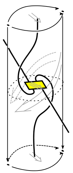
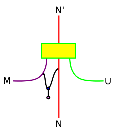
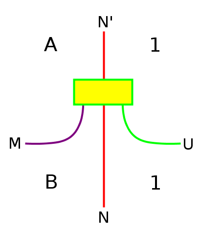
Suppose we are looking, locally, at a piece of worldsheet where “a closed string state comes in from infinity” – a bulk field insertion. Whatever that really means, following the FRS prescription we are to describe the situation by a diagram of this kind:
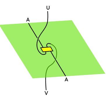
Here the plane indicates the piece of worldsheet surface which we are looking at. The rectangle in the center is the place where the bulk field is inserted.
Every such bulk field is labeled by two representations of the chiral algebra (the “left- and right-moving part”). These appear in the diagram as the two ribbons running vertically. These are to be thought of as being labeled by the (identity morphism on) the simple objects and of the modular tensor category which these representations correspond to.
The horizontal ribbon line running inside the surface is, in general, what is called a defect line. While these are important for understanding the general situation (they encode for instance dualities like T-duality or t’Hooft operators, such as appear in the 2d QFT description of geometric Langlands), let us assume for the moment that in our example this represents what is called a trivial defect, in which case this line is essentially an artefact of our description of the situation, but not itself of intrinsic meaning. Still, the FRS formalism requires that wherever we want to include a bulk field insertion such a line has to be present. Moreover, it needs to be labeled, so we are told by the FRS recipe, by a Frobenius algebra object inside the given representation category (satisfying a couple of extra properties, called “specialness”, “symmetry” and possibly, if the formalism is to be applicable also to unoriented worldsheets, “Jandl“ness).
Given these labellings, one has to furthermore consider the objects and in the modular tensor category as -bimodules with the obvious action of on itself, where we act on from the left by braiding under while we act on by braiding over . Then, finally, the coupon in the center of the diagram is to be labeled by a morphsim in the modular tensor category which is a homomorphism of internal -bimodules.
This is the FRS labelling prescription for a bulk field insertion. Similar prescriptions exist for boundary conditions and boundary field insertions.
The main motivation for considering precisely this prescription is: it works. It just so happnes that when combined with the rest of the FRS formalism, this can be shown to result in some construction which correctly describes CFT correlators with bulk insertions.
But a hint as to why this works is possibly contained in the following statement, which we now turn to:
Clue #1. The above ribbon diagram is precisely the Poincaré-dual string diagram corresponding to a cylindrical 3-morphism in the 3-category .
This 3-category is the 3-category naturally associated to any braided monoidal category:
- it has a single object
- it has one 1-morphism for each algebra object internal to
- it has one 2-morphism from to for every --bimodule internal to
- it has one 3-morphism for every bimodule homomorphism internal to .
Composition along the single object is the tensor product on which is inherited from the fact that is braided. Composition along 1-morphisms is the ordinary tensor product of bimodules and compositon along 3-morphisms is just the composition of bimodule homomorphisms.
Even though is a natural thing to consider, it may still appear like quite a mouthful to swallow. However, it turns out that is actually to be thought of as nothing but the 3-category of endomorphisms of the canonical 1-dimensional 3-vector space: this is the single object of , while the 1-morphisms in there are the “linear operators” on it, etc.
The reader not on speaking terms with internal bimodules is therefore strongly encouraged to think, in the following, of as the home of the space of states over a point of a 3-particle described by a 3-dimensional TQFT– (i.e. a membrane-like particle, as described in QFT of Charged -Particle: Extended Worldvolumes ).
In fact, for our purposes we should slightly oversimplify and think of our 3-category as being the category of 3-vector spaces. This is only slight abuse of terminology but very useful for understanding the general picture by comparison with that of ordinary (not -categorically refined ) quantum theory.
Then, what we should be considering are cylinders in . For us, a cylinder in an -category is the kind of -morphism which a transformation of -functors assigns to an -morphism of the given domain -category.
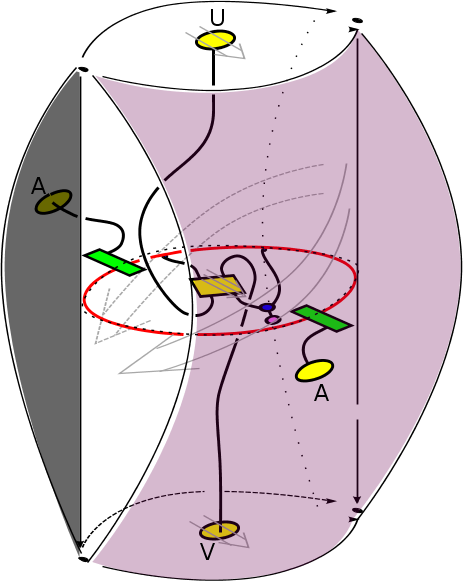
For the first few , such cylinders look like this:
(This is taken from Extended QFT and Cohomology II: Sections, States, Twists and Holography)
Here we have and hence “true 3-dimensional” cylinders.
Notice that when such cylinders really arise as components of transformations of -functors, their top and bottom are fixed to be the images of some 2-morphism under the -functors and , respectively. This is because they need to form a naturality “square” at level . For this looks like
(More details on 3-functors and their morphisms and higher morphisms are given in Picturing Morphisms of 3-Functors.)
It will turn out to be sufficient, for the present purpose, to consider a simple special case of 3-functors with values in 3-vector spaces: we can assume that they are restricted by the fact that they send every 1-morphisms to the identity.
Such cylinders in hence are labelled by
- an algebra on the left vertical seam
- an algebra on the right vertical seam
- an - bimodule on the front face
- another - bimodule on the rear face
- an - bimodule on the top
- and an - bimodule on the bottom.
Here denotes the tensor unit in , equipped with the trivial algebra structure on it. Therefore and are nothing but mere objects in !
The collection of all cylinders of this form yields an interesting 2-category in its own right. It has been described in more detail in
The 1-Dimensional 3-Vector Space
Bulk Fields and Induced Bimodules
A 3-Category of twisted Bimodules.
With the concept of a cylinder in thus established, our clue#1 is now easily checked:
the Poincaré-dual string diagram
which discribes the cylindrical 3-morphism in is precisely the type of diagram which the FRS prescription tells us to associate to a bulk field insertion:
We take this as a first indication that
The 2-dimensional theory really arises, when regarded as an extended propagation 2-functor, as a transformation of a 3-functor.
A major clue: the full disk diagram
The simplest self-contained setup which is built around the concept of a single bulk insertion, like those discussed above, is that where the bulk insertion sits on a disk-shaped worldsheet.
This requires specifying some kind of boundary condition on the rim of the disk. The FRS prescription tells us to model this boundary condition by choosing an object in the modular tensor category with the structure of an internal -module on it, for the algebra object which already appeared above, labelling the ribbon that runs inside the worldsheet. Then we are to consider the ribbon graph which has this object running in a circle, with the -line inside it, and attached with its end to the module line, where at the points these ribbons meet they are glued by those morphisms in which encode the action of on .
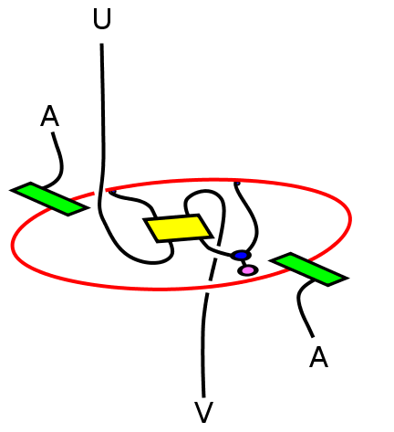
More interestingly, one can consider the situation where two “open string states come in from infinity”, i.e. where we have two boundary insertions. Whatever that really mean, in the FRS formalism this is modelled by
- choosing two (possibly different) -module objects and in , encoding the boundary conditions on the two ends of these open strings
- choosing for the two boundary field insertions morphisms and respectively.
Then instead of a single -line running around the disk we are to have and run over a semi-circle each. And where these lines meet, we are to glue them with these morphisms and .
So, in summary, the ribbon graph which the FRS prescription tells us to associate to a disk-shaped worldsheet with one bulk and two boundary field insertions looks like this:
Remarkably, for understanding the -categorical mechanism at work here in the background, it is quite helpful at this point to bring to mind the physical interpretation of this situation:
when considering the disk with two boundary insertions and we are really describing the situation where a quantum string (the “2-particle”, a linearly extended kind of particle) with quantum state propagates along its way, thereby suffering some transformations of kinds – here essentially it merges or “emits” a closed string, transforming it, schematically, into a state Finally, we probe for the “probability amplitude” that as a result of this propagation and interaction we see a string in the state running away to infinity.
A little reflection shows that this pairing of states is actually modeled after the Hom-functor:
- let be our extended QFT -functor restricted to the -categorical parameter space of the -particle which we are describing (as discussed in more detail in QFT of Charged -Particle: Extended Worldvolumes)
- let be the tensor unit of all such -functors.
Then
- a state is a morphism
- a costate is a morphism
- a (free) propagator is a morphism
Hence a pairing of states is acually an -functor
Remarkably, it turns out that the -categorical formalism knows all about the necessity of boundary conditions for extended objects, i. e. for -particles with :
for , the objects of are just complex numbers. But for , one sees that the complex numbers sit inside , but that is considerably larger.
Therefore a correlator is obtained from a pairing of states of the -particle only after we choose an -trivialization of , for the canonical inclusion of the ground field into the endomorphisms of the trivial extended -dimensional QFT, hence a morphism
It turns out that the choice of morphism here is what encodes the boundary conditions.
Since these boundary conditions are famously known, for , as “D-branes”, and since the morphism in that case, being a transformation of 2-functors, is given by 2-commuting diagrams known as tin can diagrams, the slogan is that we obtain D-branes from tin cans. This was developed in
D-Branes from Tin Cans: Arrow Theory of Disks
D-Branes from Tin Cans, Part II
D-Branes from Tin Cans, Part III: Homs of Homs
Of relevance for our purpose here is what this implies for the pairing of two states of the 3-particle:
the relation between the pairing of two states and the corresponding transformation which encodes the correlator is given by a diagram of the form
 .
.
where on the left the two cylinders appearing are to be thought of as the two 3-states of our 3-particle, the cylinder on the right is the one encoding the actual value of their correlator, while the wedge-like pieces are the modification of transformations of 3-functors coming from the morphism called above.
(A little more on such manipulations with 3-functors can be found in Picturing Morphisms of 3-Functors.)
Solving this for the cylinder on the right shows that this is given by an expression of the following form
 .
.
This indicates that the 3-morphism in which our extended QFT assigns to the disk looks like this:
As this indicates, the Poincaré dual string diagram of the 3-morphisms which describes the pairing of states of the membrane reproduces the FRS decoration prescription for a correlator of the 2-particle.
More precisely, to turn this into a well defined statement, one first needs to locally trivialize the 2-functor with respect to the canonical inclusion of the modular tensor category in the category of bimodules internal to that. Requiring the existence of such a local trivialization precisely encodes the demand that
The algebras appearing here have to be special Frobenius algebras.
Special Frobenius algebras come from special ambidextrous adjunctions, and these are what allow the local trivialization of 2-functors (see this for more).
Many of the structures appearing in the FRS formalism can actually be compared to similar structures appearing in the description of surface transport in 2-bundles with connection, by following the first edge of the cube. The reason is, we claim, that in both cases we are dealing with -functors and their local trivialization: in one case these -functors describe “classical propagation”, namely parallel transport in an -bundle with connection, in the other case they encode quantum propagation.
This close similarity becomes much more pronounced once one realizes that the local descent data for gerbes (2-bundles) is also controlled by Frobenius algebras, or rather by “Frobenius monoidoids”, only that these happen to have an invertible product operation, which makes the Frobenius property become hard to notice. (A remark on this can be found at Frobenius Algebroids with Invertible Products.)
More details on local trivialization and local description of 2-functors with values in (induced) bimodules is given in FRS Formalism from 2-Transport.
All the 2-morphisms discussed there have to be regarded as 2-dimensional cross-sections of the cylindrical 3-morphisms which we discussed so far. This then explains why they involve bimodules induced by tensoring with objects and acting by over- or underbraiding as used there.
By switching to this 2-dimensional notation, working out the local trivialization, and then finally passing from globular to string diagrams produces from our 3-morphism above finally the following planar diagram
This is the FRS disk diagram. Compare to section 4.3 of
Fuchs, Runkel, Schweigert TFT construction of RCFT correlators IV: Structure constants and correlation functions.
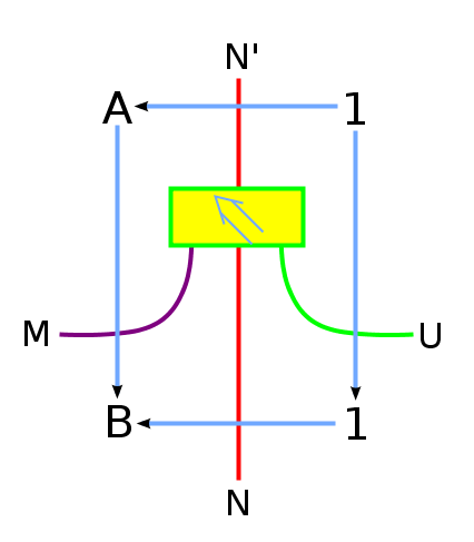
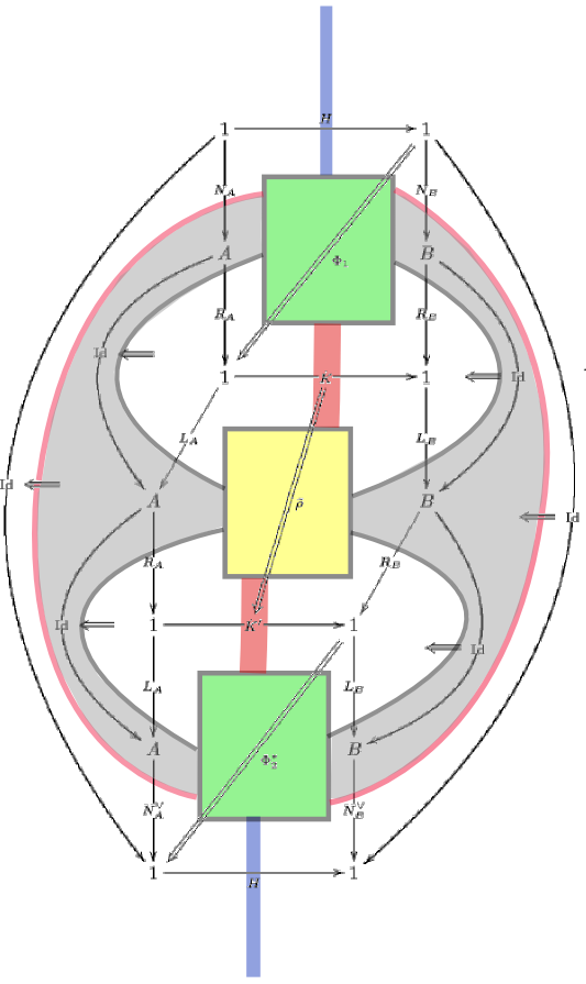
Re: QFT of Charged n-Particle: Towards 2-Functorial CFT
Here is the diagram which illustrates the horizontal composition of those cylinders (in with top and bottom rims restricted to be identities), which translates in the CFT to having two disorder lines (one taking the CFT from its -phase to its -phase, the next one taking it to its -phase) whith two bulk disorder field insertions sitting on them: