Skip to the Main Content

Note:These pages make extensive use of the latest XHTML and CSS Standards. They ought to look great in any standards-compliant modern browser. Unfortunately, they will probably look horrible in older browsers, like Netscape 4.x and IE 4.x. Moreover, many posts use MathML, which is, currently only supported in Mozilla. My best suggestion (and you will thank me when surfing an ever-increasing number of sites on the web which have been crafted to use the new standards) is to upgrade to the latest version of your browser. If that's not possible, consider moving to the Standards-compliant and open-source Mozilla browser.

June 19, 2017

The Geometric McKay Correspondence (Part 1)

Posted by John Baez

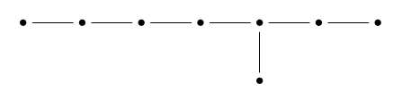
The ‘geometric McKay correspondence’, actually discovered by Patrick du Val in 1934, is a wonderful relation between the Platonic solids and the ADE Dynkin diagrams. In particular, it sets up a connection between two of my favorite things, the icosahedron:

and the E 8\mathrm{E}_8 Dynkin diagram:

When I recently gave a talk on this topic, I realized I didn’t understand it as well as I’d like. Since then I’ve been making progress with the help of this book:

  • Alexander Kirillov Jr., Quiver Representations and Quiver Varieties, AMS, Providence, Rhode Island, 2016.

I now think I glimpse a way forward to a very concrete and vivid understanding of the relation between the icosahedron and E8. It’s really just a matter of taking the ideas in this book and working them out concretely in this case. But it takes some thought, at least for me. I’d like to enlist your help.

The rotational symmetry group of the icosahedron is a subgroup of SO(3)\mathrm{SO}(3) with 60 elements, so its double cover up in SU(2)\mathrm{SU}(2) has 120. This double cover is called the binary icosahedral group, but I’ll call it Γ\Gamma for short.

This group Γ\Gamma is the star of the show, the link between the icosahedron and E8. To visualize this group, it’s good to think of SU(2)\mathrm{SU}(2) as the unit quaternions. This lets us think of the elements of Γ\Gamma as 120 points in the unit sphere in 4 dimensions. They are in fact the vertices of a 4-dimensional regular polytope, which looks like this:

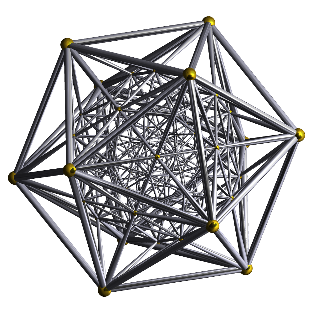
It’s called the 600-cell.

Since Γ\Gamma is a subgroup of SU(2)\mathrm{SU}(2) it acts on 2\mathbb{C}^2, and we can form the quotient space

S= 2/ΓS = \mathbb{C}^2/\Gamma

This is a smooth manifold except at the origin—that is, the point coming from 0 20 \in \mathbb{C}^2. There’s a singularity at the origin, and this where E 8\mathrm{E}_8 is hiding! The reason is that there’s a smooth manifold S˜\widetilde{S} and a map

π:S˜S\pi : \widetilde{S} \to S

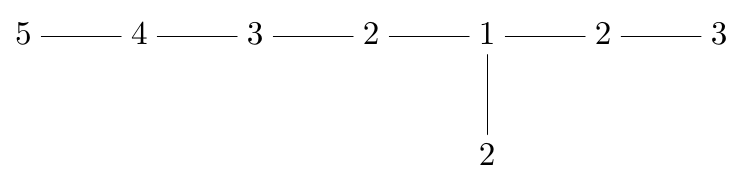
that’s one-to-one and onto except at the origin. It maps 8 spheres to the origin! There’s one of these spheres for each dot here:

Two of these spheres intersect in a point if their dots are connected by an edge; otherwise they’re disjoint.

The challenge is to find a nice concrete description of S˜\widetilde{S}, the map π:S˜S\pi : \widetilde{S} \to S, and these 8 spheres.

But first it’s good to get a mental image of SS. Each point in this space is a Γ\Gamma orbit in 2\mathbb{C}^2, meaning a set like this:

{gx:gΓ}\{g x : \; g \in \Gamma \}

for some x 2x \in \mathbb{C}^2. For x=0x = 0 this set is a single point, and that’s what I’ve been calling the ‘origin’. In all other cases it’s 120 points, the vertices of a 600-cell in 2\mathbb{C}^2. This 600-cell is centered at the point 0 20 \in \mathbb{C}^2, but it can be big or small, depending on the magnitude of xx.

So, as we take a journey starting at the origin in SS, we see a point explode into a 600-cell, which grows and perhaps also rotates as we go. The origin, the singularity in SS, is a bit like the Big Bang.

Unfortunately not every 600-cell centered at the origin is of the form I’ve shown:

{gx:gΓ}\{g x : \; g \in \Gamma \}

It’s easiest to see this by thinking of points in 4d space as quaternions rather than elements of 2\mathbb{C}^2. Then the points gΓg \in \Gamma are unit quaternions forming the vertices of a 600-cell, and multiplying gg on the right by xx dilates this 600-cell and also rotates it… but we don’t get arbitrary rotations this way. To get an arbitrarily rotated 600-cell we’d have to use both a left and right multiplication, and consider

{xgy:gΓ}\{x g y : \; g \in \Gamma \}

for a pair of quaternions x,yx, y.

Luckily, there’s a simpler picture of the space SS. It’s the space of all regular icosahedra centered at the origin in 3d space!

To see this, we start by switching to the quaternion description, which says

S=/ΓS = \mathbb{H}/\Gamma

Specifying a point xx \in \mathbb{H} amounts to specifying the magnitude x\|x\| together with x/xx/\|x\|, which is a unit quaternion, or equivalently an element of SU(2)\mathrm{SU}(2). So, specifying a point in

{gx:gΓ}/Γ\{g x : \; g \in \Gamma \} \in \mathbb{H}/\Gamma

amounts to specifying the magnitude x\|x\| together with a point in SU(2)/Γ\mathrm{SU}(2)/\Gamma. But SU(2)\mathrm{SU}(2) modulo the binary icosahedral group Γ\Gamma is the same as SO(3)\mathrm{SO}(3) modulo the icosahedral group (the rotational symmetry group of an icosahedron). Furthermore, SO(3)\mathrm{SO}(3) modulo the icosahedral group is just the space of unit-sized icosahedra centered at the origin of 3\mathbb{R}^3.

So, specifying a point

{gx:gΓ}/Γ\{g x : \; g \in \Gamma \} \in \mathbb{H}/\Gamma

amounts to specifying a nonnegative number x\|x\| together with a unit-sized icosahedron centered at the origin of 3\mathbb{R}^3. But this is the same as specifying an icosahedron of arbitrary size centered at the origin of 3\mathbb{R}^3. There’s just one subtlety: we allow the size of this icosahedron to be zero, but then the way it’s rotated no longer matters.

So, SS is the space of icosahedra centered at the origin, with the ‘icosahedron of zero size’ being a singularity in this space. When we pass to the smooth manifold S˜\widetilde{S}, we replace this singularity with 8 spheres, intersecting in a pattern described by the E 8\mathrm{E}_8 Dynkin diagram.

Points on these spheres are limiting cases of icosahedra centered at the origin. We can approach these points by letting an icosahedron centered at the origin shrink to zero size in a clever way, perhaps spinning about wildly as it does.

I don’t understand this last paragraph nearly as well as I’d like! I’m quite sure it’s true, and I know a lot of relevant information, but I don’t see it. There should be a vivid picture of how this works, not just an abstract argument. Next time I’ll start trying to assemble the material that I think needs to go into building this vivid picture.

Posted at June 19, 2017 9:30 PM UTC

TrackBack URL for this Entry:   https://golem.ph.utexas.edu/cgi-bin/MT-3.0/dxy-tb.fcgi/2968

17 Comments & 0 Trackbacks

Re: The Geometric McKay Correspondence (Part 1)

From what I understand, not being an algebraic geometer, resolutions of singularities of surfaces aren’t necessarily unique, although there should be a unique minimal resolution. Is the 8-linked-spheres one you mentioned the minimal resolution? I would assume so, since it’s part of a more general construction, but am not sure. How does this look for E7?

Posted by: Layra Idarani on June 20, 2017 4:24 AM | Permalink | Reply to this

Re: The Geometric McKay Correspondence (Part 1)

In general there is not a unique minimal resolution (they’re supposed to be related by flips). In this case it is unique.

BTW I think it’s interesting to note that the special fiber of the resolution, this Dynkin curve made of projective lines, is not generically reduced – the multiplicity of a component is the coefficient of the corresponding simple root in the expansion of the highest root (i.e. some number from 2 to 6).

Posted by: Allen Knutson on June 20, 2017 4:52 AM | Permalink | Reply to this

Re: The Geometric McKay Correspondence (Part 1)

Sorry, I haven’t been seeing notifications of comments on this post!

The space I’m calling S˜\widetilde{S} is the unique minimal resolution of 2\mathbb{C}^2 modulo the binary icosahedral group Γ\Gamma. It has 8 spheres mapping to the singular point of 2/Γ\mathbb{C}^2/\Gamma, intersecting (not linked) in a pattern given by the E 8\mathrm{E}_8 Dynkin diagram.

If we want to get the E 7\mathrm{E}_7 or E 6\mathrm{E}_6 Dynkin diagram, we just replace the binary icosahedral group by the binary octahedral or tetrahedral group. But in some ways the icosahedral case is actually the simplest! So I’ll focus on this one in my posts, and let the others fend for themselves in the comments.

Posted by: John Baez on June 25, 2017 6:56 PM | Permalink | Reply to this

Re: The Geometric McKay Correspondence (Part 1)

The tetrahedral/E6_6 case caught my eye, because a tetrahedron inscribed in the Bloch sphere is the simplest example of a symmetric informationally complete (SIC) quantum measurement. Shrinking the tetrahedron, pulling its vertices closer to the origin, yields a type of quantum measurement (sometimes designated a SIM) that has more intrinsic noise. Apparently, E6_6 is part of the story of what happens when the noise level becomes maximal and the four outcomes of the measurement merge into a single degenerate case.

Posted by: Blake Stacey on June 28, 2017 11:31 PM | Permalink | Reply to this

Re: The Geometric McKay Correspondence (Part 1)

The same thing can be done with a regular icosahedron inscribed in the Bloch sphere. Of the smattering of results known about this construction, one that I recall is that it is a tight complex projective 5-design (see Bengtsson and Zyczkowski).

Posted by: Blake Stacey on June 29, 2017 3:00 PM | Permalink | Reply to this

Re: The Geometric McKay Correspondence (Part 1)

Blake wrote:

The tetrahedral/E 6\mathrm{E}_6 case caught my eye, because a tetrahedron inscribed in the Bloch sphere is the simplest example of a symmetric informationally complete (SIC) quantum measurement. Shrinking the tetrahedron, pulling its vertices closer to the origin, yields a type of quantum measurement (sometimes designated a SIM) that has more intrinsic noise.

Excellent! Perhaps I should translate for nonphysical mathematicians, or mathematical nonphysicists:

The Bloch sphere, also known as the Riemann sphere or P 1\mathbb{C}P^1, is the space of pure states for a quantum system whose Hilbert space is 2\mathbb{C}^2 — that is, self-adjoint projection operators on this Hilbert space. This sphere is the boundary of a 3-ball, the ‘Bloch ball’, which is the space of mixed states for the same system — that is, 2×22 \times 2 nonnegative self-adjoint matrices with trace 1.

So, Blake is really considering tetrahedra inscribed in this 3-ball, centered at the origin, and seeing what happens in the limit as they shrink to zero size.

Apparently, E 6\mathrm{E}_6 is part of the story of what happens when the noise level becomes maximal and the four outcomes of the measurement merge into a single degenerate case.

Great! I feel this must be closely related to what I’m going to talk about in this series.

Here my job will be to figure out how E 8\mathrm{E}_8 shows up at the singularity in the space of all icosahedra centered at the origin of the Bloch ball… the singularity that occurs where these icosahedra shrink to zero size. But if we work with a cube or octahedron, we should see E 7\mathrm{E}_7 coming up in a similar way, and if we use a tetrahedron, we should see E 6\mathrm{E}_6.

If this story isn’t already known in the quantum information community, and you’re interested, I’d be happy to work with you to develop it. We could start by chatting on my blog articles and seeing where it goes.

Posted by: John Baez on July 2, 2017 6:36 PM | Permalink | Reply to this

Re: The Geometric McKay Correspondence (Part 1)

I don’t think the story is known in the quantum information community, so developing it in conversations here sounds like a good idea.

Here my job will be to figure out how E 8\mathrm{E}_8 shows up at the singularity in the space of all icosahedra centered at the origin of the Bloch ball… the singularity that occurs where these icosahedra shrink to zero size. But if we work with a cube or octahedron, we should see E 7\mathrm{E}_7 coming up in a similar way, and if we use a tetrahedron, we should see E 6\mathrm{E}_6.

Both the cube and the octahedron have meaning on the quantum-information side, to people who study discrete structures in finite-dimensional Hilbert spaces. The vertices of a cube can be divided up to make two tetrahedra, dual to each other; in the Bloch-ball picture, this corresponds to a pair of SICs, constructed in such a way that each vector in one SIC is orthogonal to exactly one vector in the other. (It confused me for a little while that vectors which are orthogonal to each other in the Hilbert space are antipodal to each other when represented on the Bloch sphere.) Similarly, the vertices of a regular octahedron inscribed in the Bloch sphere correspond to states which comprise a complete set of mutually unbiased bases.

Posted by: Blake Stacey on July 3, 2017 7:31 PM | Permalink | Reply to this

Re: The Geometric McKay Correspondence (Part 1)

A piece of magic that I have yet to understand connects these singularities directly with the Lie groups of the same name. Something like “consider a string moving in SS: this physical system has as its automorphism group the Lie group E 8E_8, or perhaps the loop group thereof…” The story is supposed to continue that a string, unlike a particle, doesn’t distinguish between SS and S˜\tilde S, and I guess you are supposed to see the maximal torus of E 8E_8 by certain automorphisms corresponding to the spheres in S˜\tilde S. Have you yet worked out how to picture that part of the story?

Posted by: Theo Johnson-Freyd on June 20, 2017 9:27 PM | Permalink | Reply to this

Re: The Geometric McKay Correspondence (Part 1)

I haven’t been trying to work out the string theory picture, because so far all roads to the geometric McKay correspondence that I’ve explored require that one understand the resolution π:S˜S\pi \colon \widetilde{S} \to S and its ‘exceptional fiber’, consisting of spheres intersecting in a pattern given by a Dynkin diagram.

There’s also the ‘algebraic’ McKay correspondence, which is superficially a bit different, but fundamentally the same.

Posted by: John Baez on June 27, 2017 12:00 PM | Permalink | Reply to this

Re: The Geometric McKay Correspondence (Part 1)

One can obtain a 4D quasicrystal by projecting from the E 8E_8 lattice, whose cross-section is a 3D quasicrystal with icosahedral symmetry.

See Elser and Sloane’s paper.

Posted by: Metatron on June 23, 2017 5:30 AM | Permalink | Reply to this

Re: The Geometric McKay Correspondence (Part 1)

Yes! I wrote about this in “week270” and “week271” of This Week’s Finds. The algebraic essence is a relation between noncrystallographic Coxeter diagrams with nn dots and crystallographic ones (that is, Dynkin diagrams) with 2n2n dots. This connects:

  • H 2\mathrm{H}_2 (the full symmetry group of the regular pentagon) with E 6\mathrm{E}_6,

  • H 3\mathrm{H}_3 (the full symmetry group of the icosahedron or dodecahedron) with E 7\mathrm{E}_7, and

  • H 4\mathrm{H}_4 (the full symmetry group of the 120-cell or 600-cell) with E 8\mathrm{E}_8.

This correspondence is different than the McKay correspondence linking

  • A 3\mathrm{A}_3 (the full symmetry group of the tetrahedron) with E 6\mathrm{E}_6

  • BC 3\mathrm{BC}_3 (the full symmetry group of the octahedron or cube) with E 7\mathrm{E}_7, and

  • H 3\mathrm{H}_3 (the full symmetry group of the icosahedron or dodecahedron) with E 8\mathrm{E}_8.

However, the E 8\mathrm{E}_8 cases of these two correspondences are closely connected!

Posted by: John Baez on June 27, 2017 2:31 PM | Permalink | Reply to this

Re: The Geometric McKay Correspondence (Part 1)

A very minor note: your slides refer several times to a paper by ‘Slowody’. Actually his name is ‘Slodowy’.

Posted by: L Spice on June 25, 2017 10:44 PM | Permalink | Reply to this

Re: The Geometric McKay Correspondence (Part 1)

Yikes! I’ll fix that. Thanks!

Posted by: John Baez on June 27, 2017 2:06 PM | Permalink | Reply to this

Re: The Geometric McKay Correspondence (Part 1)

I think I remember seeing somewhere a direct canonical construction of this minimal resolution S˜\tilde{S}. If so, all that would be required would be to translate it “viscerally” into the “space of icosahedra” picture.

Posted by: Bruce Bartlett on June 28, 2017 9:04 AM | Permalink | Reply to this

Re: The Geometric McKay Correspondence (Part 1)

I know a couple constructions of S˜\widetilde{S}.

In the first, we first blow up 2\mathbb{C}^2 at the origin to get a space XX, and then we resolve singularities in X/ΓX/\Gamma. In the first step the origin in 2\mathbb{C}^2 gets replaced by a Riemann sphere in XX, and the action of Γ\Gamma on this Riemann sphere factors through the obvious action of the icosahedral group on the sphere. There are thus three singularities in X/ΓX/\Gamma, coming from the vertices, edge centers and face centers in the icosahedron. Resolving these three singularities gives the three ‘legs’ in the E 8\mathrm{E}_8 Dynkin diagram:

ultimately because the vertices, edge centers and face centers have stabilizers of order 5, 2 and 3, respectively.

This is nice, but I want to understand a second more efficient construction of S˜\widetilde{S}, using the ‘equivariant punctual Hilbert scheme’ of Γ\Gamma acting on 2\mathbb{C}^2. So that’s what I’ll mainly talk about in future posts!

To understand this second construction more concretely, I’ll need to relate it to the first one. I’m hoping for your help.

Posted by: John Baez on July 2, 2017 5:17 PM | Permalink | Reply to this

Re: The Geometric McKay Correspondence (Part 1)

By the way: if you have noticed any mistakes in the book, or have some suggestions, I’d really appreciate them. Thanks! - Sasha Kirillov Jr.

Posted by: Alexander Kirillov on July 3, 2017 12:17 AM | Permalink | Reply to this

Re: The Geometric McKay Correspondence (Part 1)

I’m really enjoying your book—I took it with me to Hong Kong for a month as my only physical piece of reading material. I was focused on the material connected to the geometric McKay correspondence, but I eventually want to learn everything in this book.

I’ll keep an eye out for typos. My main suggestion is that it would be nice to have a Conclusion that summarizes the big picture, or outlines some directions for further research. I find math books a bit depressing when they suddenly end without something like this. Your last sentence is “In this case Theorem A.28 gives a complete classification of irreducible finite-dimensional representations of 𝔤\mathfrak{g}.” It’s like a glorious symphony that just stops without a finale.

Posted by: John Baez on July 4, 2017 3:45 PM | Permalink | Reply to this

Post a New Comment