A Discussion on Notions of Lawvere Theories
Posted by Emily Riehl
.")
Guest post by Daniel Cicala
The Kan Extension Seminar II continues with a discussion of the paper Notions of Lawvere Theory by Stephen Lack and Jirí Rosický.
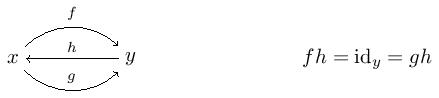
In his landmark thesis, William Lawvere introduced a method to the study of universal algebra that was vastly more abstract than those previously used. This method actually turns certain mathematical stuff, structure, and properties into a mathematical object! This is achieved with a Lawvere theory: a bijective-on-objects product preserving functor where is a skeleton of the category and is a category with finite products. The analogy between algebraic gadgets and Lawvere theories reads as: stuff, structure, and properties correspond respectively to 1, morphisms, and commuting diagrams.
To get an actual instance, or a model, of an algebraic gadget from a Lawvere theory, we take a product preserving functor . A model picks out a set and -ary operations for every -morphism .
To read more about classical Lawvere theories, you can read Evangelia Aleiferi’s discussion of Hyland and Power’s paper on the topic.
With this elegant perspective on universal algebra, we do what mathematicians are wont to do: generalize it. However, there is much to consider undertaking such a project. Firstly, what elements of the theory ought to be generalized? Lack and Rosický provide a clear answer to this question. They generalize along the following three tracks:
consider a class of limits besides finite products,
replace the base category with some other suitable category, and
enrich everything.
Another important consideration is to determine exactly how far to generalize. Why not just go as far as possible? Here are two reasons. First, there are a number of results in this paper that stand up to further generalization if one doesn’t care about constructibility. A second limiting factor of generalization is that one should ensure that central properties still hold. In Notions of Lawvere Theory, the properties lifted from classical Lawvere theories are
the correspondence between Lawvere theories and monads,
that algebraic functors have left adjoints, and
models form reflective subcategories of certain functor categories.
Before starting the discussion of the paper, I would like to take a moment to thank Alexander, Brendan and Emily for running this seminar. I have truly learned a lot and have enjoyed wonderful conversations with everyone involved.
Replacing finite limits
To find a suitable class of limits to replace finite products, we require the concept of presentability. The best entry point is to learn about local finite presentability, which David Myers has discussed here. With a little modification to the ideas there, we define a notion of local strong finite presentability and local -presentability for a class of limits .
We begin with sifted colimits, which are those -valued colimits that commute with finite products. Note the familiarity of this definition with the commutativity property of filtered colimits. Of course, filtered colimits are also sifted. Another example is a reflexive pair, that is a category with shape
Anyway, we now look at the strongly finitely presentable objects in a category . These are those objects whose representable preserves sifted colimits. Denote the full subcategory of these by . Some simple examples include , which consists of the finite sets, and , which has the free and finitely generated Abelian groups. Also, given a category of models for a Lawvere theory, is exactly those finitely presentable objects that are regular projective. A category is locally strongly finitely presentable if it is cocomplete, is small, and any -object is a sifted colimit of a diagram in . There is also a nice characterization (Theorem 3.1 in the paper) that states is locally strongly finitely presentable if and only if has finite coproducts and we can identity with the category of finite product-preserving functors . One of the most important results of Notions of Lawvere Theory, was in expanding the theory to encompass sifted (weighted) colimits. More on this later.
We can play this game with any class of limits . Before defining -presentability, here is a bit of jargon.
Definition. A functor is -flat if its colimit commutes with -limits.
We call an object of a category -presentable if preserves -flat colimits. Given the full subcategory of -presentable objects, we call locally -presentable if it is cocomplete, is small, and any -object is a -flat colimit of a diagram in . Fortunately, we retain the characterization of being locally -presentable if and only if has -colimits and is equivalent to the category - of -continuous functors . Important results in Notions of Lawvere Theory use the assumption of -presentability.
Let’s come back to Lawvere theories. From this point on, we fix a symmetric monoidal closed category that is both complete and cocomplete. Also, will refer to a class of weights over . Our first task will be to determine what class of limits can replace finite products in the classical case. To this end, we take the following assumption.
Axiom A. -continuous weights are -flat.
This axiom is an analogy with how filtered colimits commute with finite limits in . But for what classes of limits does this hold?
To answer this question, we fix a sound doctrine . Very roughly, a sound doctrine is a collection of small categories whose limits behave nicely with respect to certain colimits. After putting some small assumptions on the underlying category which we’ll sweep under the rug, define to be the full sub -category consisting of those objects such that preserves -flat colimits. Let be the class of limits ‘built from’ conical -limits and -powers in the sense that we take if
any -category with conical limits and -powers also admits -weighted limits, and
any -functor conical limits and -powers also preserves -weighted limits.
The fancy way of saying this is that is the saturation class of conical -limits and -powers. It’s easy enough to see that contains the conical -limits and -powers.
Having constructed a class of limits from a sound doctrine , we use the following theorem to imply that satisfies the axiom above.
Theorem. Let be a small -category with -weighted limits and be a -functor. The following are equivalent:
is -continuous;
is -flat
is -continuous.
In particular, the first item allows us to construct using sound limits and the equivalence between the second and third item is precisely the axiom of interest. Here are some examples.
Example. Let be the collection of all finite categories. We will also take be locally finitely presentable with the additional requirement that the monoidal unit is finitely presentable as is the tensor product of two finitely presentable objects. Examples of such a are categories of sets, abelian groups, modules over a commutative ring, chain complexes, categories, groupoids, and simplicial sets. Then , as constructed from above gives a good notion of -enriched finite limits.
Example. A second example, and one of the main contributions of Notions of Lawvere Theory is when is the class of all finite, discrete categories. Here, we take our as in the first example, though we do not require the monoidal unit to be strongly finitely presentable. We do this because, by requiring the monoidal unit to be strongly finitely presentable, we lose the example where is the category of directed graphs, which happens to be a key example, particularly to realizing categories as an model of a Lawvere theory. In this case, the induced class gives an enriched version of strongly finite limits as discussed above. This generalizes finite products in the sense that they coincide when is .
Correspondence between Lawvere theories and monads
Now that we’ve gotten our hands on some suitable limits, let’s see how we can obtain the classical correspondence between Lawvere theories and monads. Naturally, we’ll be assuming axiom A. In addition, we fix a -category that satisfies the following.
Axiom B1. is locally -presentable.
This axiom implies, as in our discussions above, that -. This is not particularly restrictive, as presheaf -categories are locally -presentable.
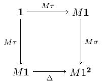
Now, define a Lawvere -theory on to be a bijective-on-objects -functor that preserves -limits. A striking difference between a Lawvere -theory and the classical notion is that the former does not require to have the limits under consideration. This makes defining the models of a Lawvere -theory a subtler issue than in the classical case. Instead of defining a model to be a -continuous functor as one might expect, we instead use the pullback square
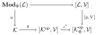
To understand what a model looks like, use the intuition for a pullback in the category and the fact that is equivalent to -. So a model will be a -functor whose restriction along is -continuous.
The other major player in this section is the category of -flat monads . We claim that there is an equivalence between and . To verify this, we construct a pair of functors between and . The first under consideration: . We define this with the help of the following proposition.
Proposition. The functor from the above pullback diagram is monadic via a -flat monad .
Hence, a -theory gives a monadic functor that yields a monad on . Moreover, this monad preserves all the limits required to be an object in . So, define .
Next, we define a functor . Consider a monad in . As per usual, factors through the Eilenberg-Moore category which we precompose with the inclusion giving . Now defining a -category that has objects from and , we factor
where is bijective-on-objects and is full and faithful. This factorization is unique up to unique isomorphism. Define .
At this point, we have functors so let’s turn our attention to showing that these are mutual weak inverses. The first step is to show that the category of algebras for a given monad is the category of models .
Theorem 6.6. The -functor restricts to an isomorphism of -categories .
This theorem gives us that . The next theorem gives us the other direction.
Theorem 6.7. There is an isomorphism .
Let’s sketch the proof. Let be a Lawvere -theory. If we denote by , we get via the factorization
where is bijective-on-objects and is fully faithful. It remains to show that .
Let’s compute the image of an -object in . For this, recall that we have - by assumption. Embedding into - gives us
This, in turn, is mapped to the left Kan extension
along (the Lawvere theory we began with). Here, we can compute that is meaning the factorization above is
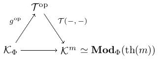
Therefore, as desired.
Many-sorted theories
Moving from single-sorted to many-sorted theories, we will take a different assumption on our -category .
Axiom B2. is a -category with -limits and such that the Yoneda inclusion has a -continuous left adjoint.
This requirement on is not overly restrictive as it holds for all presheaf -categories and all Grothendieck topoi when is . The nice thing about this assumption is that we can compute all colimits and -limits in by passing to , where they commute, then reflecting back.
Generalizing Lawvere theories here is a bit simpler than in the previous section. Indeed, call any small -category with -limits a -theory. Notice that we no longer have a bijective-on-objects functor involved in the definition. That functor forced the single-sortedness. With the functor no longer constraining the structure, we have the possibility for many sorts. Also, a -theory does have all -limits here, unlike in the single-sorted case. This allows for a much simpler definition of a model. Indeed, the category of models for a -theory is the full subcategory - of .
Presently, we are interested in generalizing two important properties of Lawvere theory to -theories. The first is that algebraic functors have left adjoints. The second is the reflectiveness of models.
Algebraic functors have left adjoints. A morphism of -theories is a -continuous -functor . Any such morphism induces a pullback -functor -- between model -categories. We call such functors -algebraic. And yes, these do have left adjoints just as in the context of classical Lawvere theories.
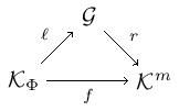
Theorem. Let and be -theories and a -functor between them. Given a model , then is a model.
What is happening here? Of course, pulling back by gives a way to turn models of into models of – this is the algebraic functor . But the left Kan extension along gives a way to turn a model of into a model of as depicted in the diagram
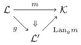
This theorem says that process gives a functor -- given by .
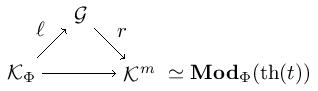
We can prove this theorem for without requiring axiom B2. This axiom is used to extend this result to a -category . The existence of the left adjoint to the Yoneda embedding of gives a factorization . The proof then reduces to showing that is -continuous, since we are already assuming that is. But because the codomain of is , we can rest on the fact that we have proven the result for . Limits are taken pointwise, after all. Actually, the left adjoint to holds more generally, but our assumptions on allow us to explicitly compute the left adjoint with left Kan extensions.
Reflexiveness of models. Having discussed left adjoints of algebraic functors, we now move on to show that categories of models - are reflexive in . Consider the free-forgetful (ordinary) adjunction
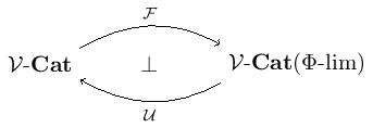
between -categories and those -categories with -limits and functors preserving them. Given a -category in the image of . Note that is a -theory. It follows from this adjunction that - is equivalent to the category . Moreover, since has -limits, the inclusion has a right adjoint inducing an algebraic functor --. But we just showed that algebraic functors have left adjoints, giving us the following theorem.
Theorem. - is reflective in .
As promised, in the two general contexts corresponding to the axioms B1 and B2, we have the Lawvere theory-monad correspondence, that algebraic functors have left adjoints, and that categories of models are reflective.
An example
After all of that abstract nonsense, let’s get our feet back on the ground. Here is an example of manifesting a category with a chosen terminal object as a generalized Lawvere theory. This comes courtesy of Nishizawa and Power.
Let denote the empty category, the terminal category, and the category with two objects and a single arrow between them. We will also take . The class of limits here is the finite -powers. We define a Lawvere -theory to be the -category where we formally add to (the opposite full subcategory on the finitely presentable objects) two arrows: and . We then close up under finite -powers and modulo the commutative diagrams
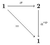
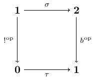
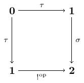
Now is the Lawvere -theory for a category with a chosen terminal object. A model of is a -continuous -functor . This means that if is a model, it must preserve powers and so the following diagrams must commute:
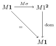
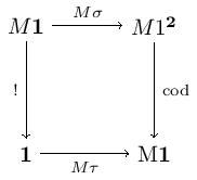
Here and choose the domain and codomain, and the diagonal functor. Note that the commutativity of these diagrams witnesses the preservation of raising the terminal category to the first three diagrams given. Let’s parse these diagrams out.
The category we get from the model is and the distinguished terminal object is chosen by . The first two diagrams provide a morphism for every object in . The third diagram gives the identity map on . The uniqueness of maps into follows from the functorality of and .
Conversely, given a category with a chosen terminal object , define a model by and for -objects . Also, let choose and let send each -object to the .
Re: A discussion on notions of Lawvere theories
Thanks for a very nice refactoring of an already nice paper.
Back when we were discussing Lawvere theories vs. monads, I got the impression that ‘finiteness’ was the main difference between monads coming from theories and arbitrary monads. But after reading your post and David’s, I now see that ‘preservation of (co)limits’ would be a better description of the difference.
(And ultimately, we can’t talk about finiteness without talking about preservation of limits)
Thanks for the example of a Lawvere theory for categories with a terminal object. In the paper you linked, they also give theories for categories with binary products and cartesian closed categories.
I was wondering if we can talk about more complicated things like abelian categories in this framework. The part about being an -enriched category with all finite limits and finite colimits is easy. But I can’t see how one would then encode the condition that all monos are kernels and all epis are cokernels.