The n-Category Café

1. Enriching over the extended real numbers

The basics

We will be thinking about enriched categories over $\overline{\mathbb{R}}\coloneqq [-\infty ,+\infty ]$, the extended real numbers. We make $\overline{\mathbb{R}}$ into a category by using the ordering $\ge$, so there is a morphism $m\to n$ if and only if $m\ge n$. (The opposite ordering is considered in Lawvere’s paper State categories, closed categories, and the existence of semi-continuous entropy functions.)

We make $\overline{\mathbb{R}}$ into a symmetric monoidal category using addition ‘$+$’ and we can use subtraction ‘$-$’ as the internal hom to make it into a closed symmetric monoidal category: this is because $$m+n\ge p\qquad \text {if and only if}\qquad m\ge p-n.$$ It’s important here to note how this arithmetic extends to the infinite elements, in particular, despite notational appearances, $-\infty$ is not the additive inverse of $+\infty$, indeed $\infty -\infty$ is a rather ambiguous thing to write as $$(+\infty )-(+\infty )=-\infty \qquad \text {and}\qquad (+\infty )+(-\infty )=+\infty .$$ Full addition and subtraction tables can be found in the nice Bachelor’s thesis of Soichiro Fujii.

We’ve got a closed symmetric monoidal category $\overline{\mathbb{R}}$ so we can consider categories enriched over $\overline{\mathbb{R}}$. An $\overline{\mathbb{R}}$-category is a generalized, generalized metric space!

Remember that a generalized metric space in the sense of Lawvere is like a metric space but the main difference is that we don’t impose that the ‘distances’ are symmetric, so in general $\mathrm{d}(x,y)\ne \mathrm{d}(y,x)$.

An $\overline{\mathbb{R}}$-category is further generalized in that we allow negative ‘distances’. For want of a better name, these generalized, generalized metric spaces I will call ‘$\overline{\mathbb{R}}$-spaces’. This means that an $\overline{\mathbb{R}}$-space is a set $X$ with a function $\mathrm{d}\colon X\times X\to \overline{\mathbb{R}}$ such that

• $0\ge \mathrm{d}(x,x)$ for all $x\in X$;

• $\mathrm{d}(x,y)+\mathrm{d}(y,z)\ge \mathrm{d}(x,z)$ for all $x,y,z\in X$.

Putting $x=y=z$ into the second inequality gives that $\mathrm{d}(x,x)$ is either $0$ or $-\infty$, with latter only possible if $\mathrm{d}(x,y)$ and $\mathrm{d}(y,x)$ are infinite for every $y\in X$.

An example of an $\overline{\mathbb{R}}$-space is $\mathbb{R}^{n}$ equipped with $\overline{\mathbb{R}}$-distance $$\mathrm{d}(x,y):=\max _{i}\{ y_{i}-x_{i}\} .$$ If you know about the Hilbert metric you might wish to think how this is related.

Vector spaces

Now suppose that we have a real vector space $V$. We think of this as a discrete $\overline{\mathbb{R}}$-spaces so that $\mathrm{d}(v,w)=+\infty$ for $v\ne w$ and $\mathrm{d}(v,v)=0$. Similarly, we think of the dual vector space $V^{#}\coloneqq \text {Hom}(V,\mathbb{R})$ as a discrete $\overline{\mathbb{R}}$-space. The tautological pairing $\langle \, ,\, \rangle \colon V\times V^{#}\to \overline{\mathbb{R}}$ can be considered as an $\overline{\mathbb{R}}$-profunctor between these $\overline{\mathbb{R}}$-spaces.

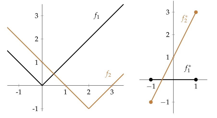
We can now interpret what the $\overline{\mathbb{R}}$-spaces of presheaves and opcopresheaves on our vector spaces are. As the vector spaces are considered as discrete $\overline{\mathbb{R}}$-metric spaces the $\overline{\mathbb{R}}$-space $\hat{V}$ of presheaves on $V$ and $\check{V^{#}}$ the $\overline{\mathbb{R}}$-space of opcopresheaves on $V^{#}$, will just be the sets of $\overline{\mathbb{R}}$-valued functions with no constraints on them, the interesting pieces of structure are the $\overline{\mathbb{R}}$ metrics: $$\begin{aligned} \mathrm{d}(f_{1},f_{2})&\coloneqq \sup _{x\in V}\{ f_{2}(x)-f_{1}(x)\} \in [-\infty ,+\infty ]\qquad \text {for all}\, \, f_{1},f_{2}\colon V\to \overline{\mathbb{R}}\\ \mathrm{d}(g_{1},g_{2})&\coloneqq \sup _{k\in V^{#}}\{ g_{1}(k)-g_{2}(k)\} \in [-\infty ,+\infty ]\qquad \text {for all}\, \, g_{1},g_{2}\colon V^{#}\to \overline{\mathbb{R}}. \end{aligned}$$ The distance from a function $f_{1}$ to a function $f_{2}$ is the most that you have to go ‘up’ from $f_{1}$ to get to $f_{2}$, where going down means going ‘up’ a negative amount.

For example, for the functions illustrated at the top of the post we have $$\mathrm{d}(f_{1},f_{2})=1,\qquad \mathrm{d}(f_{2},f_{1})=3,$$ and $$\mathrm{d}(f_{1}^{\ast },f_{2}^{\ast })=1,\qquad \mathrm{d}(f_{2}^{\ast },f_{1}^{\ast })=3.$$ The fact that these distances coincide is not mere coincidence, as we shall below.

2. The nuclear construction

Now I will remind you of the general construction of profunctor nucleus (this needs a better name!) that I blogged about last year. We start with a $\mathcal{V}$-profunctor between two $\mathcal{V}$-categories and obtain a duality between certain subcategories of presheaves on one category and copresheaves on the other. In practice, these often turn out to be interesting dualities.

For instance, if we work over the monoidal category $\{ \mathrm{true}, \mathrm{false}\}$ then a profunctor between discrete categories amounts to a relation between sets, whereas a presheaf amounts to a subset, so from a relation between between sets you get a bijection between certain distinguished sets of subsets. This underpins many dualities in mathematics. Here is a classic example.

• Suppose we take one set to be $\mathbb{C}^{n}$, the other set to be polynomials in $n$-variables, and take the relation to be that $x\in \mathbb{C}^{n}$ is related to $p\in \mathbb{C}[x_{1},\dots ,x_{n}]$ if $p(x)=0$. Then the resulting duality is the classical algebraic geometry correspondence between algebraic subsets of $\mathbb{C}^{n}$ and radical ideals of $p\in \mathbb{C}[x_{1},\dots ,x_{n}]$.

I should remind you what process leads us here. Starting with a closed symmetric category $\mathcal{V}$, two $\mathcal{V}$-categories $\mathcal{A}$ and $\mathcal{B}$, and a profunctor $$\mathcal{M}\colon \mathcal{A}^{\mathrm{op}}\otimes \mathcal{B}\to \mathcal{V}$$ between them, we obtain an adjunction between presheafs on $\mathcal{A}$ and opcopresheaves on $\mathcal{B}$. $$\mathcal{M}^{\ast }\colon \hat{\mathcal{A}}\leftrightarrows \check{\mathcal{B}}\, \colon \!\mathcal{M}_{\ast }.$$ The left and right adjoints can be given by end formulas: for instance if $p\colon \mathcal{A}^{\mathrm{op}}\to \mathcal{V}$ is a presheaf on $\mathcal{A}$ then $$(\mathcal{M}^{\ast }p)(b) = \int _{a} [p(a),\mathcal{M}(a,b)].$$ The nucleus is defined as the centre of this adjunction. This means that it consists of the induced isomorphism between the part on which the monad is an isomorphism and the comonad is an isomorphim.

3. The synthesis

We can now feed our vector space pairing in to the profunctor nucleus machine. What pops out of the machine first is an $\overline{\mathbb{R}}$-adjunction between function spaces: $$\Fun(V,\overline{\mathbb{R}})\leftrightarrows \Fun(V^{#},\overline{\mathbb{R}}).$$ We can denote both of the maps by asterisks, and we find that both of them have the same form, so for $f\colon V\to \overline{\mathbb{R}}$ a function on $V$ and $g\colon V^{#}\to \overline{\mathbb{R}}$ a function on $V^{#}$we find $$\begin{aligned} f^{\ast }(k)\coloneqq \sup _{x\in V}\big \{ \langle k,x\rangle -f(x)\big \} ;\qquad g^{\ast }(x)\coloneqq \sup _{k\in V^{#}}\big \{ \langle k,x\rangle -g(k)\big \} . \end{aligned}$$ These are, of course, precisely the Legendre-Fenchel transform and its reverse!

The standard theory of the profunctor nucleus tells us that $$f^{\ast }=f^{\ast \ast \ast }$$ and $$f\mapsto f^{\ast \ast }\, \, \text {is an idempotent operation.}$$ This means that if we restrict to the image inside $\Fun(V,\overline{\mathbb{R}})$ then we get an isomorphism. The image consists of the (lower semi-continuous) convex functions, so we get $$\Cvx(V,\overline{\mathbb{R}})\cong \Cvx(V^{#},\overline{\mathbb{R}}).$$ This is the usual Fenchel-Legendre duality.

From our machine we get a little more than this. As we have an adjunction we know that $\mathrm{d}(f^{\ast },g)=\mathrm{d}(f,g^{\ast }),$: spelling that out we have the following theorem.

Theorem: Suppose that we have functions $f\colon V\to \overline{\mathbb{R}}$ and $g\colon V^{#}\to \overline{\mathbb{R}}$ then $$\sup _{k\in V^{#}}\{ f^{\ast }(k)-g(k)\} = \sup _{x\in V}\{ g^{\ast }(x)-f(x)\} .$$

I would welcome any nice interpretation of this result!

On top of that, we know that the transform is a distance non-increasing map so we have $\mathrm{d}(f_{1},f_{2})\ge \mathrm{d}(f_{1}^{\ast },f_{2}^{\ast }),$. Spelling this out as well gives the following.

Theorem: Suppose that we have functions $f_{1},f_{2}\colon V\to \overline{\mathbb{R}}$ then $$\sup _{x\in V}\{ f_{2}(x)-f_{1}(x) \} \ge \sup _{k\in V^{#}}\{ f_{1}^{\ast }(k)-f_{2}^{\ast }(k) \} .$$

As the reverse transform is also distance non-increasing, and as we know that $f=f^{\ast \ast }$ when $f$ is convex, we get the immediate corollary that distance is preserved for convex functions.

Corollary: Suppose that we have (lower semi-continuous) convex functions $f_{1},f_{2}\colon V\to \overline{\mathbb{R}}$ then $\mathrm{d}(f_{1},f_{2})=\mathrm{d}(f_{1}^{\ast },f_{2}^{\ast })$, in other words, $$\sup _{x\in V}\{ f_{2}(x)-f_{1}(x) \} = \sup _{k\in V^{#}}\{ f_{1}^{\ast }(k)-f_{2}^{\ast }(k) \} .$$

This is illustrated by the example at the top of the post (click for a larger picture), where we have already observed that $$\mathrm{d}(f_{1},f_{2})=1=\mathrm{d}(f_{1}^{\ast },f_{2}^{\ast }),\qquad \mathrm{d}(f_{2},f_{1})=3=\mathrm{d}(f_{2}^{\ast },f_{1}^{\ast }).$$

This $\overline{\mathbb{R}}$-metric on the space of (convex) functions seems to be overlooked in literature that I’ve seen. (In many cases the distance between convex functions will be infinite.) However, people do consider the partial order $\ge$ on the set of convex functions: $f_{1}\ge f_{2}$ when $f_{1}(x)\ge f_{2}(x)$ for all $x$. The $\overline{\mathbb{R}}$-distance is a refinement of this partial order in the $f_{1}\ge f_{2}$ if and only if $\mathrm{d}(f_{1},f_{2})\le 0$.

The standard fact that the Legendre-Fenchel transform is order reversing is then a corollary of the above corollary: in other words we get that for convex functions $f_{1},f_{2}\colon V\to \overline{\mathbb{R}}$ we have $$f_{1}\ge f_{2}\quad \Leftrightarrow \quad f_{2}^{\ast }\ge f_{1}^{\ast }.$$

If anyone has seen these $\overline{\mathbb{R}}$-metrics being used in this context I’d be happy to hear about it.

Anyway, the encroachment of category theory into analysis continues…