The n-Category Café

Generalizing convexity

An important part of mathematics is choosing good generalizations. How do you know what counts as “good”? You can judge it by some subjective aesthetics: this generalization smells right, that one doesn’t. You can judge it by utility: this generalization leads to useful theorems, that one doesn’t. (But what counts as useful? Again, it’s a subjective judgement.) Sometimes you have to admit that there’s no single right generalization and embrace plurality.

There’s an unambiguous notion of convexity for subsets of Euclidean space, but there are many ways of generalizing it to other spaces. The range of generalizations available depends on what you take “space” to mean. In some of the previous generalizations of Hadwiger’s theorem, “space” is taken to mean “normed vector space”, and convexity is understood as an algebraic condition: a subset $X$ of a vector space is convex if it is closed under the operation

$$(x, y) \mapsto (1 - \lambda) x + \lambda y$$

for each $\lambda \in [0, 1]$.

We, however, are going to take “space” to mean “metric space”, so we’re going to have to understand convexity as a geometric condition. Actually, there’s more than one way to do this, and later we’ll be forced to consider two different geometric formulations of convexity. But here’s the main one we’re going to use.

Let $X$ be a metric space. A path in $X$ is a continuous map $[c, c'] \to X$, where $c \leq c'$ are real numbers. A distance-preserving path is a path that is an isometry. A metric space is geodesic if every pair of points can be joined by a distance-preserving path.

For example, a subset of $\mathbb{R}^n$ is geodesic with respect to the Euclidean metric if and only if it is convex.

This definition is intuitive geometrically, but — as Lawvere establishes in Section 8 of Taking categories seriously — it is also categorically well-motivated.

The categorical story goes like this. First we need to know that every path in a metric space has a well-defined (possibly infinite) length, and that a path $\gamma: [c, c'] \to X$ has length at least $d(\gamma(c), \gamma(c'))$, with equality iff it is distance-preserving. Now, every metric space $X = (X, d)$ can be forced to be geodesic: you keep the set of points the same, and define a new metric $\hat{d}$ by taking $\hat{d}(x, y)$ to be the shortest path-length between $x$ and $y$. (I’m glossing over a minor point here, which I’ll come back to in a moment.) This process

$$(X, d) \mapsto (X, \hat{d})$$

of “geodesic remetrization” can be made into a comonad. Indeed, it’s the density comonad of a particular functor

$$[0, \infty) \to MS.$$

Here $[0, \infty)$ is a poset under $\geq$, regarded as a category; $MS$ is the category of generalized metric spaces in the sense of Lawvere (categories enriched in $[0, \infty]$); and the functor sends $x \in [0, \infty)$ to the interval $[0, x]$ with its usual symmetric metric.

We won’t need this categorical fact in anything that follows, and I can’t say I really understand it yet. But if nothing else, it’s reassuring that our chosen notion of convexity has a sound categorical justification.

Aside:  I glossed over the point of whether the infimum $\hat{d}(x, y)$ is actually attained. It isn’t necessarily. Arguably, the notion of geodesic space is less natural than the following: a metric space $X$ is a length space if for all $x, y \in X$,

$$d(x, y) = \inf \{ length(\gamma) | paths   \gamma   from   x   to   y \}.$$

So being geodesic is a stronger condition than being a length space. Lawvere’s comonad actually forces a metric space to be a (not necessarily geodesic) length space.

But for our purposes, the difference between geodesic and length spaces doesn’t matter. That’s because of a result known as the Hopf–Rinow Theorem, which states that for a metric space in which every closed bounded subset is compact, being a length space is, in fact, equivalent to being geodesic.

Measuring subsets of a general metric space

Hadwiger’s theorem classifies the ways of measuring convex subsets of Euclidean space $\mathbb{R}^n$. We’ve just chosen a way of generalizing the term convex to an arbitrary metric space. And I’ll show you now that ways of measuring generalizes without fuss.

Fix a metric space $A$ (which in the classical situation would be $\mathbb{R}^n$ with the Euclidean metric). Write $\mathcal{K}(A)$ for the set of compact geodesic subspaces of $A$. A valuation is a function

$$\phi:\mathcal{K}(A) \to \mathbb{R}$$

such that $\phi(\emptyset) = 0$ and

$$\phi(X \cup Y) = \phi(X) + \phi(Y) - \phi(X \cap Y)$$

whenever $X, Y \in \mathcal{K}(A)$ with $X \cap Y, X \cup Y \in \mathcal{K}(A)$. It is invariant if $\phi(X) = \phi(g X)$ whenever $X \in \mathcal{K}(A)$ and $g$ is an isometry of $A$ onto itself. It is continuous if it is continuous with respect to the Hausdorff metric. (If you know what the Hausdorff metric is, great. If not, it doesn’t matter: continuity is exactly the kind of thing you’d imagine.)

A way of measuring geodesic subsets of $A$ is, formally, a continuous invariant valuation on $\mathcal{K}(A)$.

All we did here is to repeat the definitions for Euclidean space, verbatim. And just as in Euclidean space, continuous invariant valuations can be added together (pointwise) and multiplied by scalars. They therefore form a vector space, $Val(A)$, whose elements are to be thought of as the measures of size.

Every metric space $A$ therefore poses a challenge:

Describe the vector space $Val(A)$.

In general, this seems to be hard. Let’s look at some examples.

Example  Hadwiger’s theorem says that $Val(\mathbb{R}^n) \cong \mathbb{R}^{n + 1}$, where the $\mathbb{R}^n$ on the left-hand side is a metric space (with the Euclidean metric) and the $\mathbb{R}^{n + 1}$ on the right-hand side is a vector space.

We saw in Part 1 that Hadwiger’s theorem actually says a bit more. It says that $Val(\mathbb{R}^n)$ has a basis $V_0, \ldots, V_n$ in which $V_i$ is an “$i$-dimensional measure”, or formally is homogeneous of degree $i$, meaning that $V_i(t X) = t^i V_i(X)$. This description determines $V_0, \ldots, V_n$ uniquely up to scaling. With a particularly nice choice of normalization, $V_i$ is called the $i$th intrinsic volume.

Example  This one is easy. Let $A$ be a finite metric space. Then the only geodesic subsets are the empty set and singletons. A valuation $\phi$ is obliged to take value $0$ on the empty set, but can take any values on the singletons. Continuity is automatic. Invariance says that $\phi(\{g(x)\}) = \phi(\{x\})$ for any $x \in A$ and self-isometry $g$ of $A$. In other words, it says that $\phi$ is constant on each orbit of the isometry group. Hence

$$Val(A) \cong \mathbb{R}^{A/Aut(A)}$$

where $Aut(A)$ is the isometry group of $A$ and $A/Aut(A)$ is the set of orbits.

Example  If you feel like an exercise, try this. Take a circle $S^1$ and define the distance between two points to be the length of the shortest arc between them. Then show that $Val(S^1) \cong \mathbb{R}^3$. This result might seem surprising, given that $S^1$ is a quotient of $\mathbb{R}$ and $Val(\mathbb{R})$ is the smaller space $\mathbb{R}^2$.

I know almost nothing about Hadwiger-like theorems for completely arbitrary metric spaces. So let’s start to specialize.

Measuring subsets of $\ell_p^n$

We’re trying to generalize a theorem about Euclidean space $\mathbb{R}^n$. Doing it for the entire class of metric spaces, all at once, seems way too challenging, so maybe a sensible first step is to try a small class of spaces that are all quite similar to Euclidean space, and all well understood.

So: for $1 \leq p \lt \infty$, let $\ell_p^n$ denote $\mathbb{R}^n$ equipped with the metric induced by the $p$-norm:

$$d(x, y) = \Bigl( \sum_{i = 1}^n |x_i - y_i|^p \Bigr)^{1/p}$$

($x, y \in \mathbb{R}^n$). Euclidean space is $\ell_2^n$, so Hadwiger’s theorem tells us that $Val(\ell_2^n) \cong \mathbb{R}^{n + 1}$. What about the other values of $p$?

My mental picture is something like this:

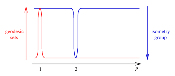
What does this mean?

• The red curve shows the size of the set $\mathcal{K}(\ell_p^n)$ of compact geodesic subsets of $\ell_p^n$. If a subset of $\mathbb{R}^n$ is convex then it’s geodesic for all values of $p$. When $p \neq 1$, the convex sets are the only geodesic subsets of $\ell_p^n$. But when $p = 1$, there turn out to be a lot more geodesic sets than just the convex ones. (We’ll come back to this.) So there’s a spike at $p = 1$.
• The blue curve shows the size of the isometry group of $\ell_p^n$. When $p \neq 2$, the isometry group of $\ell_p^n$ is very small, generated by translations, permutations of coordinates, and reflections in coordinate hyperplanes. (A coordinate subspace is a linear subspace spanned by some subset of the standard basis of $\mathbb{R}^n$; a coordinate hyperplane is an $(n-1)$-dimensional one.) The isometry group of Euclidean space $\ell_2^n$ is much bigger, since as well as permutations of coordinates you have arbitrary rotations. So there’s a spike at $p = 2$.
• The graphs are supposed to suggest how many invariant valuations there are likely to be. The more geodesic sets there are, the more valuations we expect; that’s why the $y$-axis of the red graph points upwards. The more isometries there are, the fewer invariant valuations we expect; that’s why the $y$-axis of the blue graph points downwards.
• For $p \in (1, 2) \cup (2, \infty)$, the space $\ell_p^n$ has the same geodesic subsets as $\ell_2^n$, but far fewer isometries. So we expect $Val(\ell_p^n)$ to be much bigger than $Val(\ell_2^n) \cong \mathbb{R}^{n + 1}$. (“Valuation” means the same for $\ell_p^n$ as for $\ell_2^n$, but “invariant” is a much weaker condition.) Indeed, $\Val(\ell_p^n)$ is infinite-dimensional.

But something interesting seems to be happening at $p = 1$. It’s not clear how $Val(\ell_1^n)$ will compare to $Val(\ell_2^n)$, since $\ell_1^n$ and $\ell_2^n$ have neither the same geodesic subsets nor the same isometry group. Let’s find out.

“Convex” geometry in the $1$-norm

I’ll say that a subset of $\mathbb{R}^n$ is $\ell_1$-convex if it’s geodesic when metrized as a subspace of $\ell_1^n$. Every convex set is $\ell_1$-convex, but not conversely. Here are some $\ell_1$-convex subsets of the plane:

Only the first of these is convex. The bottom-left example shows that unlike convex sets, an $\ell_1$-convex set can have different topological dimensions in different parts. If you know about reach, you can see from the two examples on the right that whereas convex sets have infinite reach, an $\ell_1$-convex set can have zero reach.

It’s probably not obvious that these sets are $\ell_1$-convex. To understand what $\ell_1$-convexity means, the following result is very helpful. In it, a path $\gamma: [c, c'] \to \mathbb{R}^n$ is called monotone if each component $\gamma_i: [c, c'] \to \mathbb{R}$ is either increasing or decreasing (in the non-strict sense).

Lemma  A subset $X \subseteq \mathbb{R}^n$ is $\ell_1$-convex if and only if every pair of points $x, y \in X$ can be joined by a monotone path in $X$.

This result, like everything else I’ll say about $\ell_1^n$, is proved here:

Tom Leinster, Integral geometry for the $1$-norm, arXiv:1012.5881.

(In its first incarnation, this paper contained several ugly, complicated proofs, and had a different title. But I managed to make it so much more simple and sleek that I decided it deserved a new name.)

The figures above suggest that the world of $\ell_1$-convex sets is much more complicated than the world of convex sets. Indeed, if you try to slavishly imitate convex geometry in the $\ell_1$ setting, something goes wrong immediately: the intersection of two $\ell_1$-convex sets need not be $\ell_1$-convex.

This should make us stop and think. Did we really choose the right generalization of convexity? Isn’t one of the fundamental properties of the class of convex sets that it’s closed under intersections? Shouldn’t we try to preserve that feature?

It turns out that things are more subtle than that. Actually, we now have to work with two different generalizations of convexity, simultaneously: being geodesic, and a kind of dual condition.

Here’s how it goes. Let $A$ be a metric space, and, for points $a$ and $b$, write $\Gamma(a, b)$ for the set of distance-preserving paths from $a$ to $b$ in $A$. A subspace $X$ of $A$ is geodesic if and only, whenever $x, y \in X$,

$$(\exists \gamma \in \Gamma(x, y))(image(\gamma) \subseteq X).$$

Dually, call $X$ cogeodesic if whenever $x, y \in X$,

$$(\forall \gamma \in \Gamma(x, y))(image(\gamma) \subseteq X).$$

In the familiar or “classical” world, Euclidean space, geodesic and cogeodesic mean the same thing: convex. The difference between the two concepts is invisible. But we see the difference in $\ell_1^n$. A subset of $\ell_1^n$ is cogeodesic if and only if it an interval, that is, a product $\prod_{i = 1}^n I_i$ where each $I_i \subseteq \mathbb{R}$ is an interval. So the situation is this:

$$\begin{matrix}   &   & Geodesic &   & Cogeodesic \\   \\ \ell_1^n: &   & \ell_1–convex &   & interval \\ \ell_2^n: &   & convex &   & convex \end{matrix}$$

The moral is that when we’re generalizing from $\ell_2^n$ to other spaces, we’re sometimes going to have to replace “convex” by “geodesic”, and sometimes by “cogeodesic”. In $\ell_1^n$, this means sometimes using $\ell_1$-convex sets and sometimes using intervals.

Let’s come back to those intersections. It’s a logical triviality that in any metric space, the intersection of a geodesic set with a cogeodesic set is geodesic. In Euclidean space, this says that the intersection of two convex sets is convex. In $\ell_1^n$, it says that the intersection of an $\ell_1$-convex set and an interval is $\ell_1$-convex. Although in one sense that’s a weaker result than we’re used to from Euclidean space, in this more subtle sense it’s precisely analogous.

Letting this principle guide us, it turns out that there are counterparts to all the standard basic results about intersections, Minkowski sums and projections of convex sets. In translating these facts from $\ell_2^n$ to $\ell_1^n$, we replace some occurrences of the word “convex” by “$\ell_1$-convex”, and others by “interval”.

All of this could be called the algebra of $\ell_1$-convex sets. There are also interesting features of the topology of the space of $\ell_1$-convex sets.

For example: in the space $\mathcal{K}(\ell_2^n)$ of ordinary convex sets, there is a dense subspace consisting of the convex polytopes. This is often used to prove theorems about all convex sets: first prove it for polytopes, then extend by continuity. Similarly, there is a class of subsets of $\mathbb{R}^n$ that I like to call the pixellated sets. Roughly, a set is pixellated if it’s a finite union of cubes with their edges parallel to the coordinate axes. (In the diagram above showing six $\ell_1$-convex sets, the top-right one is pixellated.) It can be shown that the pixellated $\ell_1$-convex sets are dense in the space $\mathcal{K}(\ell_1^n)$ of compact $\ell_1$-convex sets. This is central to the proof of the Hadwiger-type theorem for $\ell_1^n$.

Measuring subsets of $\ell_1^n$

We’re aiming to classify all ways of measuring $\ell_1$-convex sets. So far, we haven’t seen any such measures. So, our first job is to construct some.

In Euclidean space, all “measures” (continuous invariant valuations) are linear combinations of the intrinsic volumes

$$V_0, V_1, \ldots, V_n.$$

The $i$-dimensional intrinsic volume $V_i(X)$ of a set $X \in \mathcal{K}(\ell_2^n)$ is, up to a constant factor, the expected area of the projection of $X$ onto a random $i$-dimensional plane. That is, writing $Gr_{n, i}$ for the set of $i$-dimensional linear subspaces of $\mathbb{R}^n$,

$$V_i(X) = c_{n, i} \int_{Gr_{n, i}} Vol(\pi_P X)\, d P$$

where $c_{n, i}$ is a constant, $\pi_P$ is orthogonal projection onto $P$, and we’re integrating against a certain natural measure on $Gr_{n, i}$.

We want to imitate this in $\ell_1^n$.

First, how should we define the “Grassmannian” in $\ell_1^n$? This seems to require some creative thought. Whatever the $\ell_1$ Grassmannian is, let’s call it $Gr^*_{n, i}$, to distinguish it from the Euclidean Grassmannian. A key feature of the Euclidean Grassmannian $Gr_{n, i}$ is that there is no intrinsic difference between any two elements: that is, the group of origin-preserving isometries of $\ell_2^n$ acts transitively on $Gr_{n, i}$. In $\ell_1^n$, the group of origin-preserving isometries is finite, generated by coordinate permutations and reflections in coordinate hyperplanes. In order for this group to act transitively, $Gr^*_{n, i}$ had better be finite.

For this reason — and more honestly, because it turns out to work — we take $Gr^*_{n, i}$ to be the set of all $i$-dimensional coordinate subspaces of $\ell_1^n$. In other words, an element of $Gr^*_{n, i}$ is a linear subspace of $\ell_1^n$ spanned by some $i$-element subset of the standard basis.

We’ve got a natural measure on $Gr^*_{n, i}$: counting measure. Integration against counting measure is simply summation.

We can now mimic the definition of intrinsic volume. Given $i \in \{0, \ldots, n\}$ and a set $X \in \mathcal{K}(\ell_1^n)$, the $i$th $\ell_1$-intrinsic volume of $X$ is

$$V^*_i(X) = \sum_{P \in Gr^*_{n, i}} Vol(\pi_P X).$$

In principle there should be a constant factor in front of the sum, chosen to make everything work out nicely. But as it happens, the constant factor that makes everything work out nicely is $1$.

It’s a little work to show that this really is a valuation, and some more work to show that it’s continuous.

Aside:  As a clue to why continuity could be difficult, note that Lebesgue measure, as a real-valued function on the set of compact subsets of $\mathbb{R}^n$, is not continuous with respect to the Hausdorff metric. For example, take a rectangle and approximate it by a finite grid of close-together points. Then the rectangle and the finite set are close in the Hausdorff metric, but no matter how close they are, the finite set always has area zero.

It can be shown, though, that any monotone translation-invariant valuation on $\ell_1$-convex sets is continuous (by a generalization of a theorem of Peter McMullen). This tells us, in particular, that volume is continuous when restricted to $\mathcal{K}(\ell_1^n)$.

These $\ell_1$-intrinsic volumes $V^*_i$ are different from the Euclidean intrinsic volumes, even on convex sets. But they satisfy a closely analogous Hadwiger-type theorem:

Theorem:  The vector space $Val(\ell_1^n)$ of continuous invariant valuations on $\ell_1$-convex sets has dimension $n + 1$. It has a basis consisting of the $\ell_1$-intrinsic volumes $V^*_0, \ldots, V^*_n$.

A proof is given in my paper. (The $\ell_1$-intrinsic volumes are denote by $V'_i$ there, not $V^*_i$; primes don’t seem to work too well at the Café.)

The $\ell_1$-intrinsic volumes are homogeneous:

$$V^*_i(t X) = t^i V^*_i(X)$$

for any $X \in \mathcal{K}(\ell_1^n)$ and $t \gt 0$. It follows from our Hadwiger-type theorem that if $\phi$ is a continuous invariant valuation on $\mathcal{K}(\ell_1^n)$, homogeneous of degree $d$, then $d$ must belong to $\{0, \ldots, n\}$ and $\phi$ must be $V^*_d$. As Allen Knutson pointed out last time in the Euclidean context, it doesn’t seem obvious from the outset that $0, \ldots, n$ will be the only possible degrees of homogeneity; but they are.

The proof of the $\ell_1$ Hadwiger theorem relies heavily on the specifics of $\ell_1$-convex geometry, just as the classical Hadwiger theorem relies heavily on the specifics of Euclidean geometry. So it’s quite unexpected that we end up with such similar results. Note that there’s a canonical isomorphism

$$Val(\ell_1^n) \cong Val(\ell_2^n),$$

matching up $V^*_i$ with $V_i$. It’s not merely an isomorphism of vector spaces. Indeed, the vector spaces $Val(\ell_1^n)$ and $Val(\ell_2^n)$ each come equipped with an action by the multiplicative monoid $(0, \infty)$, defined by

$$(\phi t)(X) = \phi(t X)$$

whenever $\phi$ is a valuation and $t \in (0, \infty)$. The isomorphism $Val(\ell_1^n) \cong Val(\ell_2^n)$ respects that action.

Corollary:  Let $p, q \in [1, \infty)$. Then:

• if neither $p$ nor $q$ is in $\{1, 2\}$ then $Val(\ell_p^n) = Val(\ell_q^n)$ for all $n \geq 0$
• if both $p$ and $q$ are in $\{1, 2\}$ then there is a canonical isomorphism $Val(\ell_p^n) \cong Val(\ell_q^n)$ for all $n \geq 0$
• if one but not both of $p$ and $q$ is in $\{1, 2\}$ then $Val(\ell_p^n)$ and $Val(\ell_q^n)$ are not isomorphic for any $n \geq 2$.

Why do $\ell_1^n$ and $\ell_2^n$ behave so similarly to each other, yet so differently from all the other spaces $\ell_p^n$? It’s a mystery to me.

Over the horizon

There’s actually a whole lot more to the resemblance between $\ell_1^n$ and $\ell_2^n$. My paper takes some of the classic old formulas of integral geometry — Steiner’s formula, Crofton’s formula, the kinematic formulas — and reproduces them in the context of $\ell_1^n$. The new formulas are very closely analogous to the old ones, right down to the constants involved. But again, the proofs rely ultimately on geometric facts that are quite specific to the $\ell_1$ setting.

Here are some things I don’t know. Mark Meckes pointed out to me that the case $p = \infty$ would be well worth thinking about. By chance, $\ell_\infty^2$ is isometric to $\ell_1^2$, so the sequence

$$dim(Val(\ell_\infty^0)), dim(Val(\ell_\infty^1)), dim(Val(\ell_\infty^2)), \ldots$$

begins

$$1, 2, 3, \ldots,$$

which is the same as for $p = 1$ and $p = 2$. (I don’t know anything about $Val(\ell_\infty^n)$ for $n \gt 2$.) For $p \in (1, 2) \cup (2, \infty)$, the sequence is

$$1, 2, \infty, \infty, \infty, \ldots,$$

so $p = \infty$ definitely doesn’t behave like $p \in (1, 2) \cup (2, \infty)$. Whether it behaves like $p = 1$ and $p = 2$ in all dimensions is, I believe, an open question.

There’s also the case $0 \lt p \lt 1$. For $p$ in this range, the usual formula for $d(x, y)$ doesn’t define a metric, because the triangle inequality fails. However, the formula

$$d(x, y) = \sum_i |x_i - y_i|^p$$

(note the lack of $(1/p)$th power!) does define a metric, and $\mathbb{R}^n$ with this metric is called $\ell_p^n$. I don’t know anything about $Val(\ell_p^n)$ for $0 \lt p \lt 1$. Maybe the problem is trivial; I haven’t begun to think about it.