The n-Category Café

Some linear actions

Now, this series of posts is (in some sense) really about various actions of the group $PSL(2, \mathbb{Z})$ and some of its subgroups and quotients, so I want to talk about $PSL(2,\mathbb{Z})$; but I think I’ll start off by taking a step back, and talking instead about the group $SL(2,\mathbb{Z})$.

$SL(2,\mathbb{Z})$ is the group of $2\times 2$ matrices with integer entries and a determinant of $1$. For instance, $\left(\array{3&5\\7&12}\right)$, $\left(\array{1&1\\9&10}\right)$ or $\left(\array{1&-2\\-3&7}\right)$.

We can get this group to act naturally on ordered pairs of integers, by putting the pairs of integers into column vectors and multiplying them by matrices on the left. E.g.

$\left(\array{3&5\\7&12}\right)\left(\array{-4\\3}\right)=\left(\array{3\\8}\right)$.

And so forth.

We’re not restricted to acting on pairs of integers, either. Obviously, $SL(2,\mathbb{Z})$ can act in the same way on pairs of numbers from larger number systems containing the integers: for instance, pairs of rational numbers, pairs of real numbers, or pairs of complex numbers.

We can take these ordered pairs of numbers to be coordinates of a plane. For instance, here is the $\mathbb{Z}^2$ plane sitting inside the $\mathbb{R}^2$ plane. I’ve drawn some extra features as well (some lines and a square) and coloured one of the points red so we can see what happens when we act on these planes with an element of $SL(2,\mathbb{Z})$.

Acting on it with $\left(\array{2&1\\1&1}\right)$, the points get rearranged, and the lines and the blue square get sent to other lines and a blue parallelogram. In fact, we get the picture below. (I’ve left the coordinate labels in place while everything else moves under them.) The points with integer coordinates get sent to other points with integer coordinates, so we can’t tell they’ve moved without the aid of the extra features—but they have, and the black lines, blue parallelogram and red dot indicate how.

Invariants

Now, $SL(2,\mathbb{Z})$ preserves a bunch of things about the planes shown above when it acts on them. For instance, since the matrices that make up its elements have determinant $1$, the action preserves area in the plane $\mathbb{R}^2$. So the thin blue parallelogram has an area of $1$, just like the square it came from. Area is of course a geometric property associated with $\mathbb{R}^2$, but in this context we can give it an algebraic formulation, which allows us to express the area-preserving property in an equivalent way which is meaningful for $\mathbb{Z}^2$ too. For the area of a parallelogram is the magnitude of the vector cross-product of two adjacent sides.

For instance, the blue square had one side going from $(0,0)$ to $(1,0)$—the vector difference being $(1,0)$—and another going from $(0,0)$ to $(0,1)$, with vector difference $(0,1)$. In the blue parallelogram, these vectors get sent to $(2, 1)$ and $(1, 1)$.

The vector cross-product needs $3$ dimensions to work, so we add in a $z$-coordinate, and set it to $0$ in the plane. Then the vector cross-product of $(x_1, y_1, 0)$ and $(x_2, y_2, 0)$ has magnitude $\vert x_1 y_2-x_2 y_1\vert$. And, restricting to parallelograms with one vertex at the origin, we can conclude that for two points in the plane with coordinates $(x_1, y_1)$ and $(x_2, y_2)$, the quantity $\vert x_1 y_2-x_2 y_1\vert$ is preserved by the action of $SL(2,\mathbb{Z})$. Indeed, since the determinants of the matrices are $1$, the signed magnitude $x_1 y_2-x_2 y_1$ is also preserved. This algebraic quantity is of course perfectly well defined for pairs of integers. Last time, I called the coordinates by different names—instead of $(x_1, y_1)$ and $(x_2, y_2)$, I called the points $(a, c)$ and $(b, d)$. This was so I could line up the two column vectors of coordinates side by side like this:

$\left(\array{a\\c}\right)\left(\array{b\\d}\right)$

and say that the quantity $a d-b c$ is preserved, which (not coincidentally) is the determinant of the matrix $\left(\array{a&b\\c&d}\right)$. There’s a bit more to say about this, but I’ll put it off until I’ve talked about some other stuff that I need to discuss first.

So anyway, one of the things that is preserved is the vector cross-product.

A second is the vector sum:

$\left(\array{x_1\\y_1}\right)+\left(\array{x_2\\y_2}\right)=\left(\array{x_1+x_2\\y_1+y_2}\right)$

Obviously, the sum-of-vectors operation commutes with the linear transformations given by elements of $SL(2, \mathbb{Z})$.

And thirdly, the action of $SL(2,\mathbb{Z})$ preserves the property “being a line through the origin”. Indeed, we get a transitive action on the set of lines through the origin, and I want to say a bit about this next.

Lines through the origin

Lines through the origin are another geometric concept with an easy algebraic characterisation. For a line in the $\mathbb{R}^2$ plane, we pick a point $(x, y)$ on the line (other than the origin), and the line is the points $(\lambda x, \lambda y)$ for all real lambda. For lines in the $\mathbb{Z}^2$ plane, we can pick one of the points on it closest to the origin, $(m, n)$, and the line is all points $(k m, k n)$ for integer $k$.

(Of course, in the latter case there are two points closest to the origin, $(m, n)$ and $(-m, -n)$.)

Alternatively, we can characterise the lines in terms of a formal ratio of $y$ to $x$. Thus the line made of points of the form $(\lambda x, \lambda y)$ can be characterised by the ratio $\frac{y}{x}$, which is invariant under multiplication of both top and bottom by $\lambda$. For non-zero $y$, this an actual ratio—for lines in $\mathbb{R}^2$ we get a real number and for lines in $\mathbb{Z}^2$ we get a rational number. But we also have the extra line given by $\frac{1}{0}$. The lines through the origin in these planes together constitute the points on the projective lines over $\mathbb{R}$ and $\mathbb{Z}$ respectively, with $\frac{1}{0}$ being the “point at infinity”.

And as we might expect, this also works for other number systems such as $\mathbb{Q}$ and $\mathbb{C}$.

Projective invariants

Now we want to return to those invariants on $\mathbb{Z}^2$ and $\mathbb{R}^2$ (etc) that we looked at earlier, namely, for two points $(x_1, y_1)$ and $(x_2, y_2)$, the parallelogram area $x_1 y_2 - x_2 y_1$ and the sum relation $(x_1, y_1) + (x_2, y_2) = (x_1 + x_2, y_1 + y_2)$. Have these been disrupted by going from points to lines containing those points?

At this point a crucial difference arises between $\mathbb{R}$ and $\mathbb{C}$ on the one hand, and $\mathbb{Z}$ and $\mathbb{Q}$ on the other. Considering area first: replacing $(x_1, y_1)$ by $(\lambda x_1, \lambda y_1)$ has the effect of multiplying $x_1 y_2 - x_2 y_1$ by $\lambda$. So we appear to have lost our invariant.

However, for $\mathbb{Z}$ or $\mathbb{Q}$, we can still identify, and cancel out, the factors of $\lambda$, by reducing the fraction to its lowest form. This leaves only a sign ambiguity (between $(m, n)$ and $(-m, -n)$). And by picking the absolute value $\vert x_1 y_2 - x_2 y_1\vert$ coming from the reduced form of the fraction, we can get rid of the sign ambiguity too, and get an true invariant of pairs of points of the projective line. And thus for any natural number $k$, we get an invariant relation on the projective line given by picking out the pairs of points with $\vert x_1 y_2 - x_2 y_1\vert = k$. In particular, this is true of $k=1$, which is the case for which we joined the fractions by an edge last time.

Now, for the sum, we can do the same thing, reducing fractions to their lowest form, and extracting the numerator and denominator. As in the previous paragraph, there is still a sign ambiguity, so what we get is an invariant ternary relation among triplets of points, given by $\pm\mathbf{a}\pm\mathbf{b}\pm\mathbf{c}=0$. By this, I mean that, given three points $a$, $b$ and $c$ on the projective line over (say) $\mathbb{Q}$, we look at these as lines in $\mathbb{Z}^2$, take one of the two points closest to the origin on each of those lines, think of those points as position vectors $\mathbf{a}$, $\mathbf{b}$ and $\mathbf{c}$, and then fiddle with the signs of those vectors to see if any combination gives a triplet that sums to zero. If so, then this relation will be invariant under $SL(2, \mathbb{Z})$. Given any two lines, identified by the points, $\pm\mathbf{a}$ and $\pm\mathbf{b}$, there will be two lines $\pm\mathbf{c}$ which enter into such a relation with them: viz. $\pm(\mathbf{a}+\mathbf{b})$ and $\pm(\mathbf{a}-\mathbf{b})$.

So now we have our binary relation giving edges, and our ternary relation giving triangles.

Finally, we notice that $SL(2, \mathbb{Z})$ does not act freely on the lines in a plane: the matrix $\left(\array{-1&0\\0&-1}\right)$ belongs to this group, and sends $(m, n)$ to $(-m, -n)$, corresponding to the same line. This is the only non-identity matrix in $SL(2, \mathbb{Z})$ which preserves lines like this, so if we quotient $SL(2, \mathbb{Z})$ out by the subgroup $\left\{\left(\array{1&0\\0&1}\right),\left(\array{-1&0\\0&-1}\right)\right\}$, we get a free action on the projective line. And that quotient group is just the projective group $PSL(2, \mathbb{Z})$.

The complex case

Now let’s try the same thing over $\mathbb{C}$. So we take the plane consisting of pairs of complex numbers $(z, w)$. (This is not the same as the thing often called the “complex plane”—which is characterised by a single complex number for each point! The latter is two dimensional as a real manifold, but only one dimensional as a complex manifold.) We can act on this plane $\mathbb{C}^2$ with $SL(2, \mathbb{Z})$ as before.

Now take the lines in this two-complex-dimensional plane—each line being the set of points of the form $(\lambda z, \lambda w)$ for a given $z$ and $w$ and all $\lambda\in\mathbb{C}$. We can act on the set of lines with $SL(2, \mathbb{Z})$ or $PSL(2, \mathbb{Z})$, and algebraically this works in just the same way as over $\mathbb{R}$ or $\mathbb{Q}$ or $\mathbb{Z}$. As before, we can characterise the lines by formal ratios of complex numbers, which means either an actual ratio—a single complex number—or $\frac{1}{0}$, the point at infinity.

Something interesting shows up when we calculate what this action actually does to a complex number acting as a ratio, i.e. when we act on $z$ with $\left(\array{a&b\\c&d}\right)$ to get $\frac{a z+b}{c z+d}$. It turns out that although the real part of the result is a bit complicated, the imaginary part is the result is just $\frac{Im(z)}{c^2+d^2}$. That is, we divide the imaginary part of $z$ by a positive real number. And this in turn means that the upper half of the complex plane is sent to itself (as are the lower half of the complex plane, and the real line). By “plane” I now mean the plane given by a single complex number (which is a ratio)!

So we can consider the action of $PSL(2, \mathbb{Z})$ on the complex upper half-plane on its own.

Conformal and metric structures

Now we’ll take a more elementary geometric turn. A complex structure on a surface—I mean something that makes it locally look like pieces of complex plane—an example being if it’s an actual region of the complex plane—implies a conformal structure. That is, a structure that defines angles between any intersecting curves at any point. We get this, basically, because multiplication of complex numbers involves rotation—in particular, multiplication by $i$ gives a rotation by $90^\circ$. Moreover, a large class of nice functions on complex surfaces preserves the conformal structure, except possibly at some isolated points, which is why we care about it. In fact, on a surface with complex structure (a Riemann surface) the conformal structure tells us everything there is to know about its behaviour qua Riemann surface. A complex structure and a conformal structure are equivalent.

Now a conformal structure gives you somewhat less than an Riemannian metric; a Riemannian metric tells you not only angles but also distances. Of course, given a Riemannian metric, you get a conformal structure for free, by throwing away the distances and keeping the angles. Somewhat surprisingly, there’s a theorem that enables us to go in the other direction in a particularly nice way: given a Riemann surface, there’s a Riemannian metric on the surface, of constant curvature, which is geodesically complete, and which implies the conformal structure (i.e. agrees with it about all angles). And, up to a scaling factor, this metric is the unique one with these properties, on the given Riemann surface!

(Geodesically complete means that, if you travel along any geodesic in either direction from any starting point, at a constant distance per unit time, you can keep going forever. You’ll either go round and round a closed loop—as on a sphere—or head off toward infinity. So, for instance, the Euclidean plane (with its usual metric) is geodesically closed, because you can keep going forever in any direction from anywhere; but the Euclidean plane with a point removed is no longer geodesically complete, since if you travel along certain geodesics, you’ll run into the missing point after finite time, and be forced to stop.)

In particular, the upper half of the complex plane gives rise to a Riemannian metric of constant negative curvature which makes it isometric to the hyperbolic plane. The action of the group $PSL(2, \mathbb{Z})$ always preserves the conformal structure everywhere on the upper half plane, and since the hyperbolic metric is implied by the conformal structure, this group also acts as isometries of the hyperbolic plane.

Conformal structures are also sometimes nice for putting drawings of curved surfaces in books. For instance, one obviously can’t isometrically embed pieces of a sphere into the Euclidean plane, but one can do so conformally. If the sphere in question is the earth, this is particularly helpful for navigators since it preserves the relative bearing of different courses from a given location. And most of the maps you see (or should I say, the maps whose images you see) in atlases of the world are conformal. (Straight rhumb lines are better still.)

For navigators on hyperbolic seas, conformally accurate pictures are nice too. And such is the Poincaré Disc that I used last time to show the tiling of the hyperbolic plane by triangles. The whole hyperbolic plane is conformally shrunk down to an open disc, and geodesics are either diameters, or arcs of circles that intersect the boundary of the disc at right angles. I like this picture because it’s bounded, so you can see everything at once. If you prefer to see the same tilings of the upper half plane in its more conventional representation as … well … as the upper half of a plane, then they’re all over the internet. Here’s Wikipedia’s example:

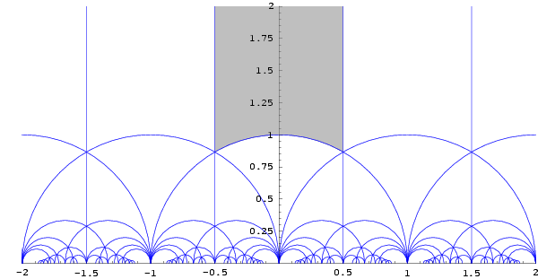
Tiled Upper Half Plane

All the figures are triangles although, as you can see, some of them have one vertex off at $\infty$, off the top of the diagram.

Now, what about when we take quotients of the hyperbolic plane by the action of $PSL(2, \mathbb{Z})$ or one of its large and interesting subgroups? What we tend to get is a surface from which protrude several long, tapering spines that stretch off to infinity without ever quite reaching a tip. So we have a noncompact surface, even if it only takes a finite number of our triangular tiles to cover it.

(The triangles are also long and tapering, and have their apices missing. This is true of every triangle when tiling the whole hyperbolic plane, but then there are an infinite number of them, so perhaps the non-compactness doesn’t seem so bothersome.)

However, there is a remedy for this.

First, throw away the Riemannian metric, but keep the conformal structure.

Now, each long, tapering spine is conformally equivalent to a disc with a point removed from its interior. So what we’ll do is mentally shrink the spines down to punctured discs, and then add an extra point to each disc to fill in the puncture. Then we paint over the new points with some topology and conformal structure, blending tastefully in with extending the existing topology and conformal structure, so it looks like new. The extra points are called cusps. And they are the apices of the triangles, and are therefore where we stick our fractions-mod-$N$ as labels.

We now have a compact surface—indeed, a compact Riemann surface. So we can imply a whole new constant-curvature, geodesically complete Riemannian metric. Adding the cusps will have changed what it takes to make the surface geodesically complete, so the new metric can be very different from the old one, and indeed need not even have negative curvature any more. Which is how we can end up with the tiled spheres that were supposed to appear at the end of the last article, as the final stage of the preceding polyhedra.

So, having explained myself, I hope, a bit more carefully than last time, I hereby present the missing spherical polyhedra. These are just the nice smooth constant-curvature versions of the dual polyhedra I showed last time.

Tetrahedron:

And now for the cube:

And finally we have the dodecahedron:

Another advantage of the spherical representation is that it enables us to properly display the tiling for $N=2$:

Let’s interpret this slightly boggolating image. There are just three reduced fractions mod $2$, viz. $\frac{1}{0}$, $\frac{0}{1}$ and $\frac{1}{1}$. These form a mediant triplet, so it looks as though the tiling mod $2$ consists of a single triangle. However, it is better to think of this as two triangles back-to-back. This is a bit silly as a polyhedron, but on the sphere, each “face” forms a different hemisphere, with the three “edges” forming three segments of the equator. This isn’t the picture shown above. Rather, dually, we get a segmentation of the sphere into three bigons, each labelled by one of the fractions—like some kind of mutant orange—and that’s what we see above.

Note that rotating around $\frac{1}{0}$ still adds $1$, and rotating around the edge between $\frac{1}{0}$ and $\frac{0}{1}$ still sends $q\rightarrow\frac{-1}{q}$, even though these operations are almost confusingly simple at this point.

We could even go to $N=1$, but the resulting single triangle, even drawn on a sphere, is rather degenerate and so I shan’t bother (it isn’t a simple monohedron, though such things exist on the sphere—it’s a triangle folded back on itself to look like a simple monohedron).

I hope that makes things a bit clearer.

Next time, we’ll look at $N>5$.