The n-Category Café

Physicists often say things like this:

“Special relativity reduces to Newtonian mechanics as the speed of light, $c$, approaches $\infty$.”

“Quantum mechanics reduces to classical mechanics as Planck’s constant $\hbar$ approaches $0$.”

“General relativity reduces to special relativity as Newton’s constant $G$ approaches $0$.”

Sometimes they try to elaborate this further with a picture called Bronstein’s cube or the CGh cube:

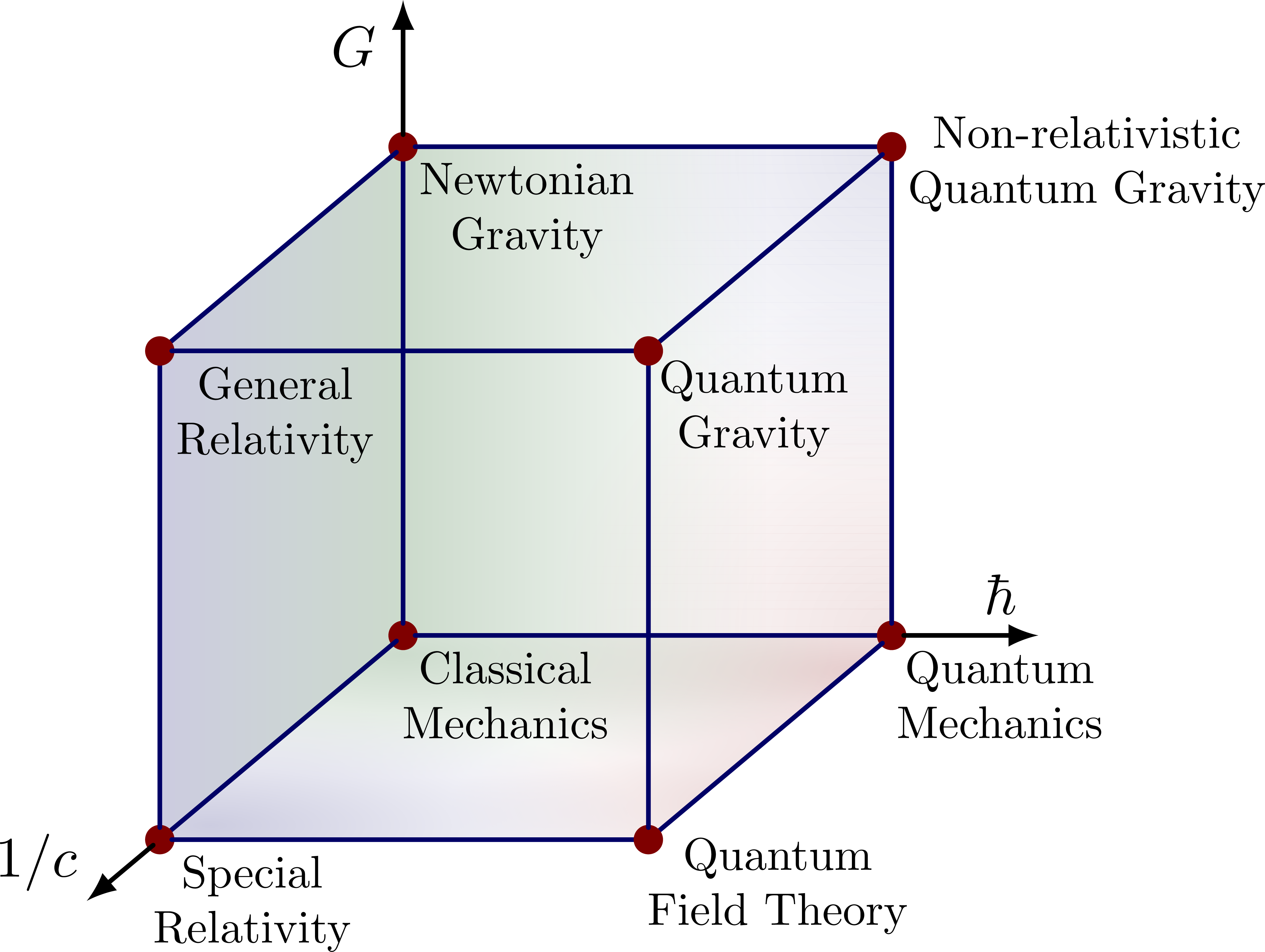
This is presumably hinting at some 3-dimensional space where $1/c, \hbar$ and $G$ can take arbitrary nonnegative values. This would be an example of what I mean by a ‘moduli space of physical frameworks’.

But right now I want to talk about talk about a fourth dimension that’s not in this cube. I want to talk about whether classical statistical mechanics reduces to thermodynamics as $k \to 0$, where $k$ is Boltzmann’s constant.

Since thermodynamics and statistical mechanics are often taught in the same course, you may be wondering how I distinguish them. Here are my two key principles: anything that involves probability theory or Boltzmann’s constant I will not call thermodynamics: I will call it statistical mechanics. For example, in thermodynamics we have quantities like energy $E$, entropy $S$, temperature $T$, obeying rules like

$$d E = T d S$$

But in classical statistical mechanics $E$ becomes a random variable and we instead have

$$d \langle E \rangle = T d S$$

In classical statistical mechanics we can also compute the variance of $E$, and this is typically proportional to Boltzmann’s constant. As $k \to 0$, this variance goes to zero and we’re back to thermodynamics! Also, in classical statistical mechanics entropy turns out to be given by

$$S = - k \int_X p(x) \ln(p(x)) \, d\mu(x)$$

where $p$ is some probability distribution on some measure space of states $(X,\mu)$.

I want to flesh out how classical statistical mechanics reduces to thermodynamics as $k \to 0$, and my hope is that this is quite analogous to how quantum mechanics reduces to classical mechanics as $\hbar \to 0$:

taking the $\hbar \to 0$ limit of	taking the $k \to 0$ limit of
Quantum Mechanics	Classical Statistical Mechanics
gives	gives
Classical Mechanics	Thermodynamics

Here’s the idea. Quantum fluctuations are a form of randomness inherent to quantum mechanics, described by complex amplitudes. Thermal fluctuations are a form of randomness inherent to classical statistical mechanics, described by real probabilities. Planck’s constant $\hbar$ sets the scale of quantum fluctuations, and as $\hbar \to 0$ these go away and quantum mechanics reduces to classical mechanics. Boltzmann’s constant $k$ sets the scale of thermal fluctuations, and as $k \to 0$ these go away and classical statistical mechanics reduces to thermodynamics.

If this idea works, the whole story for how quantum mechanics reduces to classical mechanics as $\hbar \to 0$ may be a Wick rotated version of how classical statistical mechanics reduces to thermodynamics as $k \to 0$. In other words, the two stories may be formally the same if we replace $k$ everywhere with $i \hbar$.

However, there are many obstacles to getting the idea to to work — or at least apparent obstacles, much as walls can feel like ‘obstacles’ when you’re trying to walk through a wide open door at night. Even before we meet the technical problems with Wick rotation, there’s the preliminary problem of getting thermodynamics to actually arise as the $k \to 0$ limit of classical statistical mechanics!

So despite the grand words above, it’s that preliminary problem that I’m focused on now. It’s actually really interesting.

Today I’ll just give a bit of background.

The math: deformation of rigs

Deformation quantization, is a detailed analysis of how quantum mechanics reduces to classical mechanics as $\hbar \to 0$, and how you can try to reverse this process. If you’ve thought about this a lot, may have bumped into ‘idempotent analysis’: a version of analysis where you use minimization as a replacement for addition of real numbers, and addition as a replacement for multiplication. This works because addition distributes over minimization:

$$x + (y \, \min \, z) = (x + y) \, \min \, (x + z)$$

and it’s called ‘idempotent’ because minimization obeys

$$x \, \min \, x = x$$

When we use minimization as addition we don’t get additive inverses, so numbers form a rig, meaning a ‘ring without negatives’. You also need to include $+\infty$ to serve as an additive identity for minimization.

Idempotent analysis overlaps with ‘tropical mathematics’, where people use this number system, called the ‘tropical rig’, to simplify problems in algebraic geometry. People who do idempotent analysis are motivated more by applications to physics:

• Grigory L. Litvinov, Tropical mathematics, idempotent analysis, classical mechanics and geometry.

The basic idea is to study a 1-parameter family of rigs $R_\beta$ which for finite $\beta \gt 0$ are all isomorphic to $(-\infty,\infty]$ with its usual addition and multiplication, but in the limit $\beta \to +\infty$ approach a rig isomorphic to $[0,\infty)$ with ‘min’ as addition and the usual $+$ as multiplication.

Let me describe this in more detail, so you can see exactly how it works. In classical statistical mechanics, the probability of a system being in a state of energy $E$ decreases exponentially with energy, so it’s proportional to

$$e^{-\beta E}$$

where $\beta \gt 0$ is some constant we’ll discuss later. Let’s write

$$f_\beta(E) = e^{-\beta E}$$

but let’s extend $f_\beta$ to a bijection

$$f_\beta: (-\infty, \infty] \to [0,\infty)$$

sending $\infty$ to $0$. This says that states of infinite energy have probability zero.

Now let’s conjugate ordinary addition and multiplication, which make $[0,\infty)$ into a rig, by this bijection $f_\beta$:

$$x \oplus_\beta y = f_\beta^{-1} (f_\beta(x) + f_\beta(y))$$   $$x \odot_\beta y = f_\beta^{-1} (f_\beta(x) \cdot f_\beta(y))$$

These conjugated operations make $(-\infty,\infty]$ into a rig. Explicitly, we have

$$x \oplus_\beta y = -\frac{1}{\beta} \ln(e^{-\beta x} + e^{-\beta y})$$   $$x \odot_\beta y = x + y$$

So the multiplication is always the usual $+$ on $(-\infty,\infty]$ — yes, I know this is confusing — while the addition is some more complicated operation that depends on $\beta$. We get different rig structures on $(-\infty,\infty]$ for different values of $\beta \gt 0$, but these rigs are all isomorphic because we got them all from the same rig structure on $[0,\infty)$.

However, now we can take the limit as $\beta \to +\infty$ and get operations we call $\oplus_\infty$ and $\odot_\infty$. If we work these out we get

$$x \oplus_\infty y = x \min y$$   $$x \odot_\infty y = x + y$$

These give a rig structure on $(-\infty,\infty]$ that’s not isomorphic to any of those for finite $\beta$. This is the tropical rig.

(Other people define the tropical rig differently, using different conventions, but usually theirs are isomorphic to this one.)

The physics: classical statistical mechanics

What does all of this mean for classical statistical mechanics? The idea is that $[0,\infty)$ with its usual $+$ and $\times$ is the rig of unnormalized probabilities. I’ll assume you know why we add probabilities for mutually exclusive events and multiply probabilities for independent events. But probabilities lie in $[0,1]$, which is not closed under addition. To get a rig, we work instead with ‘unnormalized’ probabilities, which lie in $[0,\infty)$. We add and multiply these just like probabilities. When we have a list of unnormalized probabilities $p_1, \dots, p_n$, we can convert them to probabilities by dividing each one by their sum. We do this normalization only after all the addition and multiplication is done and we want to make predictions.

In classical statistical mechanics, a physical system has many states, each with its own energy $E \in (-\infty,\infty]$. The unnormalized probability that the system is in a state of energy $E$ is

$$f_\beta(E) = e^{-\beta E}$$

The case of infinite energy is not ordinarily considered, but it’s allowed by the the math here, and this gives an unnormalized probability of zero.

We can reason with these unnormalized probabilities using addition and multiplication — or, equivalently, we can work directly with the energies $E$ using the operations $\oplus_\beta$ and $\odot_\beta$ on $(-\infty,\infty]$.

In short, we’ve enhanced the usual machinery of probability theory by working with unnormalized probabilities, and then transferred it over to the world of energies.

The physical meaning of $\beta \to +\infty$

All very nice. But what’s the physical meaning of $\beta$ and the $\beta \to +\infty$ limit? This is where things get tricky.

First, what’s $\beta$? In physics we usually take

$$\beta = \frac{1}{k T}$$

where $T$ is temperature and $k$ is Boltzmann’s constant. Boltzmann’s constant has units of energy/temperature — it’s about $1.38 \cdot 10^{-23}$ joules per kelvin — so in physics we use it to convert between energy and temperature. $k T$ has units of energy, so $\beta$ has units of 1/energy, and $\beta E$ is dimensionless. That’s important: we’re only allowed to exponentiate dimensionless quantities, and we want $e^{-\beta E}$ to make sense.

One can imagine doing physics using some interpretation of the deformation parameter $\beta$ other than $1/k T$. But let’s take $\beta$ to be $1/k T$. Then we can still understand the $\beta \to +\infty$ limit in more than one way! We can

1. hold $k$ constant and let $T \to 0$
2. hold $T$ constant and let $k \to 0$.

We could also try other things, like simply letting $k$ and $T$ do whatever they want as long as their product approaches zero. But let’s just consider these two options.

Hold $k$ constant and let $T \to 0$

This option seems to make plenty of sense. It’s called Boltzmann’s ‘constant’, after all. So maybe we should hold it constant and let $T$ approach zero. In this case we’re taking the low temperature limit of classical statistical mechanics.

It’s sad that we get the tropical rig as a low-temperature limit: it should have been called the arctic rig! But the physics works out well. At temperature $T$, systems in classical statistical mechanics minimize their free energy $E - T S$ where $E$ is energy and $S$ is entropy. As $T \to 0$, free energy reduces to simply the energy, $E$. Thus, in the low temperature limit, such systems always try to minimize their energy! In this limit we’re doing classical statics: the classical mechanics of systems at rest.

These ideas let us develop this analogy:

taking the $\hbar \to 0$ limit of	taking the $T \to 0$ limit of
Quantum Mechanics	Classical Statistical Mechanics
gives	gives
Classical Mechanics	Classical Statics

Blake Pollard and I explored this analogy extensively, and discovered some exciting things:

• Quantropy:

  • Part 1: the analogy between quantum mechanics and statistical mechanics, and the quantum analogue of entropy: quantropy.

  • Part 2: computing the quantropy of a quantum system starting from its partition function.

  • Part 3: the quantropy of a free particle.

  • Part 4: a paper on quantropy, written with Blake Pollard.

But while this analogy is mathematically rigorous and leads to new insights, it’s not completely satisfying. First, $\hbar$ and $T$ just feel different. Planck’s constant takes the same value everywhere while temperature is something we can control. It would be great if next to the thermostat on your wall there was a little box where you could adjust Planck’s constant, but it just doesn’t work that way!

Second, there’s a detailed analogy between classical mechanics and thermodynamics, which I explored here:

• Classical mechanics versus thermodynamics:

  • Part 1: Hamilton’s equations versus the Maxwell relations.

  • Part 2: the role of symplectic geometry.

  • Part 3: a detailed analogy between classical mechanics and thermodynamics.

  • Part 4: what is the analogue of quantization for thermodynamics?

Most of this was about how classical mechanics and thermodynamics share common mathematical structures, like symplectic and contact geometry. These structures arise naturally from variational principles: principle of least action in classical mechanics, and the principle of maximum entropy in thermodynamics. By the end of this series I had convinced myself that thermodynamics should appear as the $k \to 0$ limit of some physical framework, just as classical mechanics appears as the $\hbar \to 0$ limit of quantum mechanics. So, let’s look at option 2.

Hold $T$ constant and let $k \to 0$

Of course, my remark about holding $k$ constant because it’s called Boltzmann’s constant was just a joke. Planck’s constant is a constant too, yet it’s very fruitful to imagine treating it as a variable and letting it approach zero.

But what would it really mean to let $k \to 0$? Well, first let’s remember what it would mean to let $\hbar \to 0$.

I’ll pick a specific real-world example: a laser beam. Suppose you’re a physicist from 1900 who doesn’t know quantum mechanics, who is allowed to do experiments on a beam of laser light. If you do crude measurements, this beam will look like a simple solution to the classical Maxwell equations: an electromagnetic field oscillating sinusoidally. So you will think that classical physics is correct. Only when you do more careful measurements will you notice that this wave’s amplitude and phase are a bit ‘fuzzy’: you get different answers when you repeatedly measure these, no matter how good the beam is and how good your experimental apparatus is. These are ‘quantum fluctuations’, related to the fact that light is made of photons.

The product of the standard deviations of the amplitude and phase is bounded below by something proportional to $\hbar$. So, we say that $\hbar$ sets the scale of the quantum fluctuations. If we could let $\hbar \to 0$, these fluctuations would become ever smaller, and in the limit the purely classical description of the situation would be exact.

Something similar holds with Boltzmann’s constant. Suppose you’re a physicist from 1900 who doesn’t know about atoms, who has somehow been given the ability to measure the pressure of a gas in a sealed container with arbitrary accuracy. If you do crude measurements, the pressure will seem to be a function of the temperature, the container’s volume, and the amount of gas in the container. This will obey the laws of thermodynamics. Only when you do extremely precise experiments will you notice that the pressure is fluctuating. These are ‘thermal fluctuations’, caused by the gas being made of molecules.

The variance of the pressure is proportional to $k$. So, we say that $k$ sets the scale of the thermal fluctuations. If we could let $k \to 0$, these fluctuations would become ever smaller, and in the limit the thermodynamics description of the situation would be exact.

The analogy here is a bit rough at points, but I think there’s something to it. And if you examine the history, you’ll see some striking parallels. Einstein discovered that light is made of photons: he won the Nobel prize for his 1905 paper on this, and it led to a lot of work on quantum mechanics. But Einstein also wrote a paper in 1905 showing how to prove that liquid water is made of atoms! The idea was to measure the random Brownian motion of a grain of pollen in water — that is, thermal fluctuations. In 1908, Jean Perrin carried out this experiment, and he later won the Nobel “for his work on the discontinuous structure of matter”. So the photon theory of light and the atomic theory of matter both owe a lot to Einstein’s work.

Planck had earlier introduced what we now call Planck’s constant in his famous 1900 paper on the quantum statistical mechanics of light, without really grasping the idea of photons. Remarkably, this is also the paper that first introduced Boltzmann’s constant $k$. Boltzmann had the idea that entropy was proportional to the logarithm of the number of occupied states, but he never estimated the constant of proportionality or gave it a name: Planck did both! So Boltzmann’s constant and Planck’s constant were born hand in hand.

There’s more to say about how to correctly take the $\hbar \to 0$ limit of a laser beam: we have to simultaneously increase the expected number of photons, so that the rough macroscopic appearance of the laser beam remains the same, rather than becoming dimmer. Similarly, we have to be careful when taking the $k \to 0$ limit of a container of gas: we need to also increase the number of molecules, so that the average pressure remains the same instead of decreasing.

Getting these details right has exercised me quite a bit lately. This is what I want to talk about.