The n-Category Café

People often summarize this theorem by saying “symmetries give conservation laws”. And that’s right, but it’s only true under some assumptions: for example, that the equations of motion come from a Lagrangian.

This leads to some interesting questions. For which types of physical theories do symmetries give conservation laws? What are we assuming about the world, if we assume it is described by a theories of this type? It’s hard to get to the bottom of these questions, but it’s worth trying.

We can prove versions of Noether’s theorem relating symmetries to conserved quantities in many frameworks. While a differential geometric framework is truer to Noether’s original vision, my paper studies the theorem algebraically, without mentioning Lagrangians.

Now, Atiyah said:

…algebra is to the geometer what you might call the Faustian offer. As you know, Faust in Goethe’s story was offered whatever he wanted (in his case the love of a beautiful woman), by the devil, in return for selling his soul. Algebra is the offer made by the devil to the mathematician. The devil says: I will give you this powerful machine, it will answer any question you like. All you need to do is give me your soul: give up geometry and you will have this marvellous machine.

While this is sometimes true, algebra is more than a computational tool: it allows us to express concepts in a very clear and distilled way. Furthermore, the geometrical framework developed for classical mechanics is not sufficient for quantum mechanics. An algebraic approach emphasizes the similarity between classical and quantum mechanics, clarifying their differences.

In talking about Noether’s theorem I keep using an interlocking trio of important concepts used to describe physical systems: ‘states’, ‘observables’ and `generators’. A physical system has a convex set of states, where convex linear combinations let us describe probabilistic mixtures of states. An observable is a real-valued quantity whose value depends—perhaps with some randomness—on the state. More precisely: an observable maps each state to a probability measure on the real line. A generator, on the other hand, is something that gives rise to a one-parameter group of transformations of the set of states—or dually, of the set of observables.

It’s easy to mix up observables and generators, but I want to distinguish them. When we say ‘the energy of the system is 7 joules’, we are treating energy as an observable: something you can measure. When we say ‘the Hamiltonian generates time translations’, we are treating the Hamiltonian as a generator.

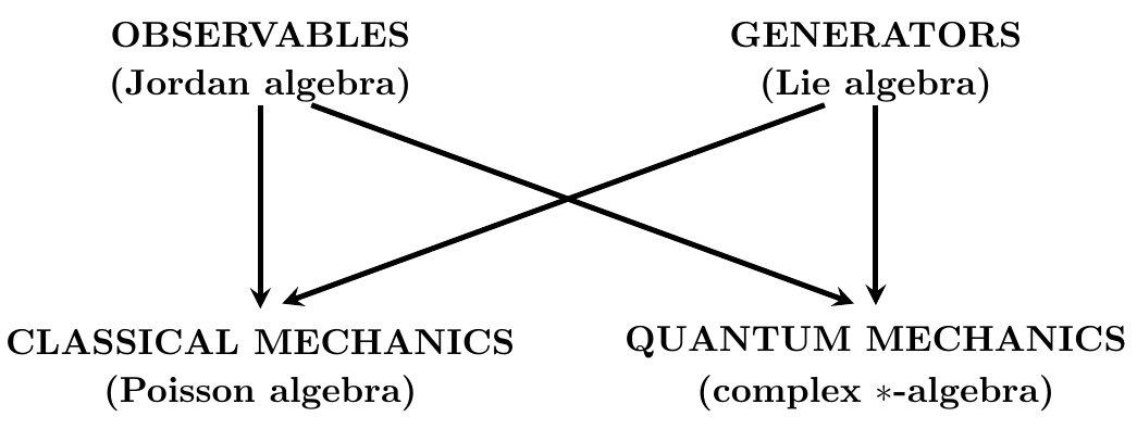
In both classical mechanics and ordinary complex quantum mechanics we usually say the Hamiltonian is the energy, because we have a way to identify them. But observables and generators play distinct roles—and in some theories, such as real or quaternionic quantum mechanics, they are truly different. In all the theories I consider in my paper the set of observables is a Jordan algebra, while the set of generators is a Lie algebra. (Don’t worry, I explain what those are.)

When we can identify observables with generators, we can state Noether’s theorem as the following equivalence:

$$The \; generator \; a \; generates \; transformations \; that \; leave \; the observable \; b \; fixed\!.$$

$$\Updownarrow$$

$$The \; generator \; b \; generates \; transformations \; that \; leave \; the \; observable \; a \; fixed\!.$$

In this beautifully symmetrical statement, we switch from thinking of $a$ as the generator and $b$ as the observable in the first part to thinking of $b$ as the generator and $a$ as the observable in the second part. Of course, this statement is true only under some conditions, and the goal of my paper is to better understand these conditions. But the most fundamental condition, I claim, is the ability to identify observables with generators.

In classical mechanics we treat observables as being the same as generators, by treating them as elements of a Poisson algebra, which is both a Jordan algebra and a Lie algebra. In quantum mechanics observables are not quite the same as generators. They are both elements of something called a ∗-algebra. Observables are self-adjoint, obeying

$$a^* = a$$

while generators are skew-adjoint, obeying

$$a^* = -a$$

The self-adjoint elements form a Jordan algebra, while the skew-adjoint elements form a Lie algebra.

In ordinary complex quantum mechanics we use a complex ∗-algebra. This lets us turn any self-adjoint element into a skew-adjoint one by multiplying it by $\sqrt{-1}$. Thus, the complex numbers let us identify observables with generators! In real and quaternionic quantum mechanics this identification is impossible, so the appearance of complex numbers in quantum mechanics is closely connected to Noether’s theorem.

In short, classical mechanics and ordinary complex quantum mechanics fit together in this sort of picture:

To dig deeper, it’s good to examine generators on their own: that is, Lie algebras. Lie algebras arise very naturally from the concept of ‘symmetry’. Any Lie group gives rise to a Lie algebra, and any element of this Lie algebra then generates a one-parameter family of transformations of that very same Lie algebra. This lets us state a version of Noether’s theorem solely in terms of generators:

$$The \; generator \; a \; generates \; transformations \; that \; leave \; the \; generator \; b fixed\!.$$

$$\Updownarrow$$

$$The \; generator \; b \; generates \; transformations \; that \; leave \; the \; generator \; a \; fixed\!.$$

And when we translate these statements into equations, their equivalence follows directly from this elementary property of the Lie bracket:

$$[a,b] = 0$$

$$\Updownarrow$$

$$[b,a] = 0$$

Thus, Noether’s theorem is almost automatic if we forget about observables and work solely with generators. The only questions left are: why should symmetries be described by Lie groups, and what is the meaning of this property of the Lie bracket?

In my paper I tackle both these questions, and point out that the Lie algebra formulation of Noether’s theorem comes from a more primitive group formulation, which says that whenever you have two group elements $g$ and $h$,

$$g \; commutes \; with h\!.$$

$$\Updownarrow$$

$$h \; commutes \; with \; g\!.$$

That is: whenever you’ve got two ways of transforming a physical system, the first transformation is ‘conserved’ by second if and only if the second is conserved by the first!

However, observables are crucial in physics. Working solely with generators in order to make Noether’s theorem a tautology would be another sort of Faustian bargain. So, to really get to the bottom of Noether’s theorem, we need to understand the map from observables to generators. In ordinary quantum mechanics this comes from multiplication by $i$. But this just pushes the mystery back a notch: why should we be using the complex numbers in quantum mechanics?

For this it’s good to spend some time examining observables on their own: that is, Jordan algebras. Those of greatest importance in physics are the unital JB-algebras, which are unfortunately named not after me, but Jordan and Banach. These allow a unified approach to real, complex and quaternionic quantum mechanics, along with some more exotic theories. So, they let us study how the role of complex numbers in quantum mechanics is connected to Noether’s theorem.

Any unital JB-algebra $O$ has a partial ordering: that is, we can talk about one observable being greater than or equal to another. With the help of this we can define states on $O,$ and prove that any observable maps each state to a probability measure on the real line.

More surprisingly, any JB-algebra also gives rise to two Lie algebras. The smaller of these, say $L,$ has elements that generate transformations of $O$ that preserve all the structure of this unital JB-algebra. They also act on the set of states. Thus, elements of $L$ truly deserve to be considered ‘generators’.

In a unital JB-algebra there is not always a way to reinterpret observables as generators. However, Alfsen and Shultz have defined the notion of a ‘dynamical correspondence’ for such an algebra, which is a well-behaved map

$$\psi \colon O \to L$$

One of the two conditions they impose on this map implies a version of Noether’s theorem. They prove that any JB-algebra with a dynamical correspondence gives a complex ∗-algebra where the observables are self-adjoint elements, the generators are skew-adjoint, and we can convert observables into generators by multiplying them by $i$.

This result is important, because the definition of JB-algebra does not involve the complex numbers, nor does the concept of dynamical correspondence. Rather, the role of the complex numbers in quantum mechanics emerges from a map from observables to generators that obeys conditions including Noether’s theorem!

To be a bit more precise, Alfsen and Shultz’s first condition on the map $\psi \colon O \to L$ says that every observable $a \in O$ generates transformations that leave $a$ itself fixed. I call this the self-conservation principle. It implies Noether’s theorem.

However, in their definition of dynamical correspondence, Alfsen and Shultz also impose a second, more mysterious condition on the map $\psi$. I claim that that this condition is best understood in terms of the larger Lie algebra associated to a unital JB-algebra. As a vector space this is the direct sum

$$A = O \oplus L$$

but it’s equipped with a Lie bracket such that

$$[-,-] \colon L \times L \to L \qquad [-,-] \colon L \times O \to O$$

$$[-,-] \colon O \times L \to O \qquad [-,-] \colon O \times O \to L$$

As I mentioned, elements of $L$ generate transformations of $O$ that preserve all the structure on this unital JB-algebra. Elements of $O$ also generate transformations of $O,$ but these only preserve its vector space structure and partial ordering.

What’s the meaning of these other transformations? I claim they’re connected to statistical mechanics.

For example, consider ordinary quantum mechanics and let $O$ be the unital JB-algebra of all bounded self-adjoint operators on a complex Hilbert space. Then $L$ is the Lie algebra of all bounded skew-adjoint operators on this Hilbert space. There is a dynamical correpondence sending any observable $H \in O$ to the generator $\psi(H) = i H \in L,$ which then generates a one-parameter group of transformations of $O$ like this:

$$a \mapsto e^{i t H/\hbar} \, a \, e^{-i t H/\hbar} \qquad \forall t \in \mathbb{R}, a \in O$$

where $\hbar$ is Planck’s constant. If $H$ is the Hamiltonian of some system, this is the usual formula for time evolution of observables in the Heisenberg picture. But $H$ also generates a one-parameter group of transformations of $O$ as follows:

$$a \mapsto e^{-\beta H/2} \, a \, e^{-\beta H/2} \qquad \forall \beta \in \mathbb{R}, a \in O$$

Writing $\beta = 1/k T$ where $T$ is temperature and $k$ is Boltzmann’s constant, I claim that these are ‘thermal transformations’. Acting on a state in thermal equilibrium at some temperature, these transformations produce states in thermal equilibrium at other temperatures (up to normalization).

The analogy between $i t/\hbar$ and $1/k T$ is often summarized by saying “inverse temperature is imaginary time”. The second condition in Alfsen and Shultz’s definition of dynamical correspondence is a way of capturing this principle in a way that does not explicitly mention the complex numbers. Thus, we may very roughly say their result explains the role of complex numbers in quantum mechanics starting from three assumptions:

• observables form Jordan algebra of a nice sort (a unital JB-algebra)

• the self-conservation principle (and thus Noether’s theorem)

• the relation between time and inverse temperature.

I still want to understand all of this more deeply, but the way statistical mechanics entered the game was surprising to me, so I feel I made a little progress.

I hope the paper is half as fun to read as it was to write! There’s a lot more in it than described here.