The n-Category Café

Weightings: functions, measures and distributions

Readers of this blog who are familiar with the idea of magnitude will be familiar with the idea of weightings. A weighting for a finite metric space is a function $w\colon A\to \mathbb{R}$ such that $$\sum _{x\in A} w(x) e^{-\mathrm{d}(x,y)} =1\quad \text{for all}\quad y\in A;$$ the magnitude is defined to be the total weight, $\left |A\right | \coloneqq \sum _{x} w(x)$. The ‘intuition’ I gave for this is that you can think of each point as a body — such as a penguin — which is giving out heat which falls off exponentially with distance, and each body — or penguin — wishes to receive a single unit of heat. The magnitude is the total heat required.

You can think about trying to extend this to infinite metric spaces such as the unit interval; a good class of metric spaces to consider is that of compact subsets of Euclidean spaces. For $X$ a compact subspace of Euclidean space there are many equivalent ways to define magnitude such as

• $\sup (\left | A\right | \colon A\subset X, A\,\, \text {finite})$

• $\lim \left |A_{n}\right |$ whenever $A_{n} \to X$ in the Hausdorff topology with each $A_{n}$ finite.

You can calculate the magnitude of the length $L$ interval using either of these and find that the answer is $L/2+1$.

It would be natural at this point to generalize the idea of a weighting from the finite situation and to guess that another way to define magnitude of such a space would be in terms of a weight measure, so that would be a signed measure $\mu$ on $X$ such that $$\int _{x} e^{-\mathrm{d}(x,y)}\, \mathrm{d}\mu =1\quad \text {for all }\,\,y\in X,$$ with the magnitude given by $\left |X\right | = \int _{x}\mathrm{d}\mu$. When such a thing exists on $X$ then it gives the same answer as the two definitions above, however, there is not always a weight measure.

You might suppose that you could just take the limit of weightings on finite subsets to get such a thing, but an important point is that the limit of finitely supported signed measures which converge pointwise is not always a signed measure.

It took me a while to get my head around this until I found the following example. Define the sequence $(\mu _{i})_{i=0}^{\infty }$ of finitely supported signed measures on the real line $\mathbb{R}$ by $\mu _{i}\coloneqq i\delta _{0} - i\delta _{1/i}$, where $\delta_x$ is the Dirac delta measure supported at $x$. Then the sequence converges pointwise because $$\int _{\mathbb{R}} f \mathrm{d}\mu _{i} = \frac{f(0)-f(1/i)}{1/i} \to f'(0)\qquad \text {as}\qquad i\to \infty .$$ But the functional $f\mapsto f'(0)$ is not represented by any signed measure. Rather it is a distribution.

A distribution on $\mathbb{R}^{n}$ here means a linear functional on some suitable class of functions on $\mathbb{R}^{n}$, say smooth and decaying appropriately to zero at $\infty$. I will be vague as I want to skip the technicalities. We would write $w$ for a distribution and its evaluation on a function $f$ as a pairing $\langle w, f\rangle$.

Here are a few of examples of distributions.

• For each (appropriately integrable) function $g$ we have an associated distribution with $\langle g, f\rangle \coloneqq \int _{\mathbb{R}^{n}} g(x)f(x) \mathrm{d} x$.

• For each signed measure $\mu$ we have an associated distribution with $\langle \mu , f\rangle \coloneqq \int _{\mathbb{R}^{n}} f \mathrm{d} \mu$.

• Generalizing the derivative mentioned above, for any (cooriented) smooth, codimension one submanifold $S$ of $\mathbb{R}^{n}$ we have the distribution $\hat{S}$ given by $$\langle \hat{S}, f\rangle \coloneqq \int _{S} \frac{\partial f(x)}{\partial \nu } \mathrm{d} x$$ where $\frac{\partial }{\partial \nu }$ means derivative in the normal direction to the submanifold.

Now we define a weight distribution to be a distribution $w$ such that $$\langle w, e^{-d(\cdot , y)}\rangle =1\quad \text {for all } y\in X.$$ Mark showed that every compact subset of Euclidean space has a weight distribution and that the magnitude of such a subset is given by $$|X| =\langle w, 1\rangle$$ where $1$ represents any function which is identically equal to $1$ on $X$.

Mark showed that having a weight distribution on a subset of Euclidean space corresponds to having a ‘potential function’. I will look at what such a thing is for the example of the $1$-ball.

The $1$-ball

Consider $B^{1}_{R}\subset \mathbb{R}$, the $1$-ball of radius $R$: this is just a length $2R$ interval with the usual metric on it. This does have a weight measure on it: $$w= \tfrac{1}{2}(\delta _{-R}+\delta _{R} + \mu )$$ where $\mu$ is the usual Lebesgue measure, while $\delta _{-R}$ and $\delta _{R}$ are Dirac delta functions on the end-points of the interval. You can do the calculation (or look in my paper) to find that $$\int _{x\in B_{R}^{1}} e^{-\mathrm{d}(x,y)}\, \mathrm{d} w =1\quad \text {for all }y\in B_{R}^{1},$$ and as $|B_{R}^{1}|=\int _{B_{R}^{1}} dw$ it is immediate that $|B_{R}^{1}|=R+1$.

We are thinking of the interval as sitting inside the real line: $B_{R}^{1}\subset \mathbb{R}^{1}$, so we can ask how much heat an infinitesimal test penguin would feel if it were not part of the main huddle that is sitting on the interval. Define the potential function $h\colon \mathbb{R}^{1} \to \mathbb{R}$ by $$h(y)\coloneqq \int _{x\in B_{R}^{1}} e^{-\mathrm{d}(x,y)}\, \mathrm{d} w$$

By the definition of $w$ we know that $h\equiv 1$ on $B_{R}^{1}$, and by a calculation we find $$h(y) =\begin{cases} e^{-R+y} &\text {for }y\lt -R\\ 1 &\text {for }-R\le y\le R\\ e^{R-y} &\text {for }R\lt y \end{cases}$$

Here is a graph of $h$.

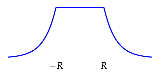
And here are some facts worth collecting about $h$.

1. $h\equiv 1$ on $B_{R}^{1}$
2. $h - h''=0$ on $\mathbb{R}\backslash B_{R}^{1}$
3. $h(x)\to 0$ as $x\to \infty$
4. $h$ is continuous (but not everywhere differentiable)

Fact (2) is the only one that doesn’t leap out from the graph, but it should be clear from the formula once it has been pointed out.

The nice thing is that these facts uniquely determine $h$. We know by (1) what $h$ is on the interval $[-R, R]$. To find it on the interval $(R,\infty )$, consider by (2) the differential equation $h''-h =0$; this is a second order linear ordinary differential equation so has a two-dimensional space of solutions, spanned by $e^{x}$ and $e^{-x}$. The former tends to infinity as $x\to \infty$, so (3) implies $h$ has to be a multiple of $e^{-x}$. We have by (1) that $h(R)=1$, so continuity at $x=R$ by (4) will fix the multiple. A similar argument works for $h$ on $(-\infty , -R)$.

We will see later on in the post that the idea that these four facts characterize the potential function actually generalizes to arbitrary compact, convex sets in odd dimensions.

Now look a little more closely at the differential equation (2) satisfied by $h$. Write $\Delta h\coloneqq h''$ as we will be wanting to consider this as the Laplacian operator on the line, and write $I$ for the identity function. The following is saying that the weighting on the $1$-ball can be recovered from its potential.

Proposition. The potential function and the weighting distribution are related on the whole of the real line by $$\tfrac{1}{2}(I-\Delta )h = w\quad \text {in the weak sense.}$$

You first need to understand what ‘in the weak sense’ means in order to understand the proposition, because $(I-\Delta )h(x)$ is certainly not defined at $x=R$ as $h$ is not differentiable there. Firstly observe that $I$ and $\Delta$ are self-adjoint with respect to the pairing on smooth functions so: $$\int _{x\in \mathbb{R}}(I-\Delta )f(x)\cdot g(x)\, \mathrm{d}x =\int _{x\in \mathbb{R}}f(x)\cdot (I-\Delta )g(x)\, \mathrm{d}x.$$ for suitably smooth and suitably decaying functions $f$ and $g$. We can write this as $$\langle (I-\Delta )f, g\rangle = \langle f, (I-\Delta )g\rangle .$$ We then say that for $h$ a not-necessarily-smooth function and $w$ a distribution that $(I-\Delta )h = w$ in the weak sense if $$\langle h, (I-\Delta ) g\rangle = \langle w, g\rangle .$$ For all suitably smooth and suitably decaying functions $g$.

You can check explicitly by hand, using integration by parts and the fundamental theorem of calculus that for the $h$ and $w$ on $\mathbb{R}$ given above, this is true.

More general subsets of Euclidean space

Look now at generalizing some of the above ideas. Let $X\subset \mathbb{R}^{n}$ be a compact set. We consider a pair consisting of a function $h$ — the potential function — and a distribution $w$ — the weighting distribution — with $$h(y) =\langle w, e^{-\mathrm{d}(\cdot ,y)} \rangle$$ such that $h\equiv 1$ on $X$ and $w\equiv 0$ off $X$.

Mark showed that such a pair always exists and used the Fourier transform to express $w$ in terms of $h$. Recall first that the Laplacian $\Delta$ on $\R^n$ is the differential operator given in usual coordinates by $\sum_{i=1}^n \frac{\partial^2}{\partial x_i^2}$.

Proposition. The potential and the weighting are related on $\mathbb{R}^{n}$ by $$\tfrac{1}{n!\, \omega _{n}}(I-\Delta )^{\frac{n+1}{2}}h = w\quad \text {in the weak sense,}$$ where $\omega_n$ is the volume of the $n$ ball.

You should be a bit worried by this in the case that $n$ is even and be asking what is meant by the fractional power of a differential operator. The short answer is that it is a pseudo-differential operator, defined via Fourier transforms, but we are not going to concern ourselves with such things here as we will concentrate on the case that $n$ is odd.

This means that the magnitude can actually be recovered directly from the potential function as $$\begin{aligned} |X|&=\langle w, 1\rangle = \langle w, h\rangle =\tfrac{1}{n!\, \omega _{n}} \langle h, (I-\Delta )^{\frac{n+1}{2}}h\rangle \\ &=\tfrac{1}{n!\, \omega _{n}}\int _{\mathbb{R}^{n}}h\cdot (I-\Delta )^{\frac{n+1}{2}}h. \end{aligned}$$

Actually, there’s a better formula than this in Tom and Mark’s survey paper (although this formula was not in the literature before). Provided that the potential function is integrable we have a particularly simple expression for the magnitude in terms of the potential function: $$|X|=\tfrac{1}{n!\, \omega _{n}}\int _{\mathbb{R}^{n}}h.$$

Tony Carbery and Juan Antonio Barceló are able to completely characterize the potential function for convex subsets of odd-dimensional Euclidean space in the following way, which generalizes the set of facts we had about the potential function of the $1$-ball above.

Proposition. Suppose $n$ is odd. The potential function $h$ for a compact, convex subset $K\subset \mathbb{R}^{n}$ satisfies the following properties and is uniquely determined by them.

1. $h\equiv 1$ on $K$
2. $(I-\Delta )^{\frac{n+1}{2}}h=0$ on $\mathbb{R}^{n}\backslash K$
3. $h(x)\to 0$ as $x\to \infty$
4. $h$ is $(n-1)/2$ times differentiable

So in this situation of convex subsets in odd dimensions, one can calculate magnitude without thinking about weightings or distributions at all. Tony and Juan Antonio use this to give an algorithm for computing the magnitude of odd dimensional balls as we will now see.

Computing the potential function of odd balls

We are interested in the $R$ radius $n$-ball, $B_{R}^{n}\subset \mathbb{R}^{n}$, where $n$ is an odd, positive integer. Tony and Juan Antonio took advantage of the symmetry. The potential function $h\colon \mathbb{R}^{n}\to \mathbb{R}$ can be taken to be spherically symmetric, so we will think of it as a function $h(r)$ of a single variable, the radial coordinate, hopefully this abuse of notation will not cause confusion. By the formula for the Laplacian in spherical coordinates, the Laplacian of a function $f(r)$ of the radius can be written in the following way. $$\Delta f(r) = f''(r) - \tfrac{n-1}{r} f'(r).$$ From the characterization of the potential function described above, this means that to find a potential function for the ball $B_{R}^{n}$ you are left with the task of finding a function $h\colon [0,\infty )\to \mathbb{R}$ such that the following hold.

1. $h(r)\equiv 1$ for $r\le R$
2. $(I+\tfrac{n-1}{r}\tfrac{\mathrm{d}}{\mathrm{d}r}- \tfrac{\mathrm{d}^{2}}{\mathrm{d}r^{2}})^{\frac{n+1}{2}}h(r)=0$ for $r\gt R$
3. $h(r)\to 0$ as $r\to \infty$
4. $h$ is $(n-1)/2$ times differentiable

Condition (2) is a homogeneous, order $n+1$, linear ODE, and so has an $n+1$ dimensional space of solutions. Tony and Juan Antonio wrote down an explicit basis of functions (these functions are related to modified spherical Bessel functions). However, $(n+1)/2$ of these tend to infinity and the other $(n+1)/2$ tend to zero. So by (3) we are left with an $(n+1)/2$-dimensional space of possible solutions. The differentiability condition (4) when $r=R$, together with (1), gives us exactly $(n+1)/2$ conditions which allows us to pin down the potential function $h$ precisely.

The potential $h$ can then be used to calculate the magnitude of the odd balls.

Payoff: the magnitude of odd balls

The above gives us an algorithm for calculating the magnitude $|B^{n}_{R}|$ when $n$ is odd. Tony and Juan Antonio do calculations for hand for $n=3, 5, 7$ (although it is not difficult to implement the algorithm in something like Sage or Maple). They get $$|B^{3} _{R}| = \frac{1}{3!} \, (R^{3} + 6R^{2} + 12 R + 6)$$ which is exactly as was predicted by the Convex Magnitude Conjecture. However, they also get $$|B^{5} _{R}| = \frac{R^{6} + 18 \, R^{5} + 135 \, R^{4} + 525 \, R^{3} + 1080 \, R^{2} + 1080 \, R + 360}{5! \, \left (R + 3\right )}$$ which is not a polynomial (!) and so gives a counterexample to the conjecture. This magnitude does, however, have the conjectured behaviour as $R\to \infty$ and as $R\to 0$, this is a consequence of some general facts proved in the paper, confirming aspects of the conjecture.

Afterword

Inspired by Carbery and Barceló’s results, I set about trying to find the magnitude of odd balls just by using weightings, without using potential theory. This gives rise to a particularly appealing explicit formula for $|B^{n}_{R}|$. Unfortunately my result relies on an integral identity that I can’t prove, but I have posted it on Mathoverflow, so do go over and see if you can help. I will undoubtably say more about this in a future post.