Skip to the Main Content

Note:These pages make extensive use of the latest XHTML and CSS Standards. They ought to look great in any standards-compliant modern browser. Unfortunately, they will probably look horrible in older browsers, like Netscape 4.x and IE 4.x. Moreover, many posts use MathML, which is, currently only supported in Mozilla. My best suggestion (and you will thank me when surfing an ever-increasing number of sites on the web which have been crafted to use the new standards) is to upgrade to the latest version of your browser. If that's not possible, consider moving to the Standards-compliant and open-source Mozilla browser.

February 12, 2015

Can a Computer Solve Lebesgue’s Universal Covering Problem?

Posted by John Baez

Here’s a problem I hope we can solve here. I think it will be fun. It involves computable analysis.

To state the problem precisely, recall that the diameter of a set of points AA in a metric space is

diam(A)=sup{d(x,y):x,yA} diam(A)=\sup\{d(x,y) : x,y\in A\}

Recall that two subsets of the Euclidean plane 2\mathbb{R}^2 are isometric if we can get one from the other by translation, rotation and/or reflection.

Finally, let’s define a universal covering to be a convex compact subset KK of the Euclidean plane such that any set A 2A \subseteq \mathbb{R}^2 of diameter 11 is isometric to a subset of KK.

In 1914 Lebesgue posed the puzzle of finding the universal covering with the least area. Since then people have been using increasingly clever constructions to find universal coverings with smaller and smaller area.

My question is whether we need an unbounded amount of cleverness, or whether we could write a program to solve this puzzle.

There are actually a number of ways to make this question precise, but let me focus on the simplest. Let 𝒰\mathcal{U} be the set of all universal coverings. Can we write a program that computes this number to as much accuracy as desired:

a=inf{area(K):K𝒰}? a=inf\{ area(K) : K \in \mathcal{U}\} \; ?

More precisely, is this real number aa computable?

Right now all we know is that

0.832a0.844115376859 0.832 \le a \le 0.844115376859\dots

though Philip Gibbs has a heuristic argument for a better lower bound:

0.84408a 0.84408 \le a

I recently wrote a letter to Greg Egan in which by the end I’d convinced myself that the answer is yes, the number aa is computable. Instead of taking the time to polish up this letter into a nice blog article, I’ll just copy it here with minimal changes. There are lots of things that need to be clarified, but I think it would be fun to do this by having a conversation here. By the end of the conversation, maybe we’ll have a theorem.

So:

Let 𝒳\mathcal{X} be the space of convex compact sets in the plane having area 1 and center of mass at the origin. There’s a function

f:𝒳[0,) f : \mathcal{X} \to [0,\infty)

sending each such set KK to the largest value of DD such that any subset of the plane with diameter DD is isometric to a subset of KK. The Lebesgue covering problem is equivalent to finding the supremum of the function ff. In particular, the number aa is computable iff the number

s=sup{f(K):K𝒳} s = sup \{f(K) :K \in \mathcal{X} \}

is computable. I guess

a=1s 2 a = \frac{1}{s^2}

or something like that.

We can put a metric on 𝒳\mathcal{X}, namely the usual Hausdorff metric. I’m willing to guess that ff is continuous with respect to this metric.

In fact, don’t think we lose anything by restricting attention to sets in the plane that lie in a ball of radius 1000: there are sets in 𝒳\mathcal{X} without this property, but they’ll be long and skinny, so they won’t maximize ff.

So, let’s redefine 𝒳\mathcal{X} to include this extra requirement: it only contains sets that lie in a ball of radius 1000. Then 𝒳\mathcal{X} will be compact! This follows from the Blaschke selection theorem.

So now

f:𝒳[0,) f: \mathcal{X} \to [0, \infty)

is a continuous function on a compact metric space. So it must be bounded and attain its supremum somewhere.

So far this is just a proof that the Lebesgue universal covering problem has a solution: there exists a universal covering of minimal area.

The next question is whether we can compute the maximum value of ff.

There’s a general fact, I believe: we can compute the maximum value of any computable function on a computably compact space. I don’t have any books on computable analysis at hand, but someone must have proved a theorem like this. We can’t compute where the maximum occurs, but we can compute the maximum value.

So, the question is just whether ff is computable.

First, what does it mean for a function

f:𝒳 f : \mathcal{X} \to \mathbb{R}

to be computable? There are some different choices of definition here, since there are different approaches to computable analysis. I guess my favorite is this. I will define what it means for

f:XY f : X \to Y

to be computable whenever XX and YY are separable metric spaces equipped with a computability structure that is, a countable dense sequence of points whose distances to each other can be computed to arbitrary desired accuracy.

Suppose x ix_i is the computability structure for XX and y jy_j is the computability structure for YY. Then ff is computable if the set of triples i,j,ni, j, n for which

d(f(x i),y j)<1/n d(f(x_i), y_j) &lt; 1/n

is recursively enumerable — that is, it can be listed by some computer program.

In our example, we will take the computability structure on \mathbb{R} to be any computable enumeration of the rationals: any way of listing the rationals that you can do with a computer program. We take the computability structure x ix_i of 𝒳\mathcal{X} to be any computable enumeration of the polygons whose vertices have rational coordinates.

The definition of computability may sound a bit complicated. The basic idea is roughly that if we can compute f(x i)f(x_i) as a function of ii, to whatever accuracy we want, our function

f:𝒳 f : \mathcal{X} \to \mathbb{R}

will be computable in the technical sense above.

Actually that’s not quite right, in general! If ff changes very rapidly in an unpredictable way, we might be able to compute it as accurately as we want for the points x ix_i but still be in the dark about nearby points. But I think we’ll be okay if two properties hold:

ff is sequentially computable: we can write a program that given ii and nn computes a rational number within 1/n1/n of f(x i)f(x_i).

ff is computably uniformly continuous: as a function of n>0n &gt; 0 we can compute m>0m &gt; 0 such that if

d(x,y)<1/m d(x,y) &lt; 1/m

then

|f(x)f(y)|<1/n |f(x) - f(y)| &lt; 1/n

If our function ff has both these properties, I believe it will be computable in the technical sense. Moreover it’s also computable in another intuitive sense.

Namely: to specify a point xXx \in X in a computable way, you have to give me a program that for each m>0m &gt; 0 will give me an ii such that

d(x i,x)<1/m d(x_i, x) &lt; 1/m

Suppose you do this, and I want to compute f(x)f(x) to accuracy 2/n2/n. First I compute mm such that

d(x,y)<1/m d(x,y) &lt; 1/m

implies

|f(x)f(y)|<1/n |f(x) - f(y)| &lt; 1/n

Then I compute f(x i)f(x_i) to an accuracy of 1/n1/n. Then by the above inequality I know f(x)f(x) to within 2/n2/n.

Now, back to our example. I believe we can show that the function in our example is computably uniformly continuous: changing the shape of a set just a little won’t dramatically change the maximum diameter DD such that it contains an isometric copy of any set of diameter DD. I bet we have something pretty simple, like

d(x,y)<1/n d(x,y) &lt; 1/n

implies

|f(x)f(y)|<1/n |f(x) - f(y)| &lt; 1/n

So the question boils down to whether ff is sequentially computable: can we compute f(x i)f(x_i) as a function of ii, to any desired accuracy?

In short: can we in principle write a program that, given a convex polygon with rational vertices, computes to any desired accuracy the largest value of DD such that any set of diameter DD can be moved, by rigid motion, until it fits inside this polygon?

This sounds hard.

However, we probably don’t need to think about “any set of diameter dd”. It’s probably enough to think about “any polygon of diameter dd with rational vertices”.

It still seems hard to tell if all these can be translated and rotated/reflected in a way that fits them inside our chosen polygon. A completely brute-force search using some discretized approximation should settle the question for any one such shape — at least “up to a specified error ϵ\epsilon”, which is not a problem here. But going through all such shapes seems hard.

Hmm, but maybe not! We can probably assume without loss of generality that these shapes are convex — and then they, too, are points in a computably compact metric space, again thanks to Blaschke’s selection theorem. So maybe I don’t need to check infinitely many such shapes can be translated, rotated or reflected to fit inside my chosen polygon. I can do it for finitely many: enough that any such shape is very close to the ones I’ve checked.

I probably should say what a ‘computably compact metric space’ is. There’s probably a standard definition of this, but I think for my purposes this will do: it’s a separable metric space XX with a computability structure such that we can write a program that given any n>0n &gt; 0 as input will list a finite set i 1,,i ki_1, \dots, i_k such that every xXx \in X is distance at most 1/n1/n from one of the points x i 1,,x i kx_{i_1}, \dots, x_{i_k}.

I believe, but haven’t proved, that the space 𝒳\mathcal{X} is computably compact.

So, right now I feel that

s=sup{f(K):K𝒳} s = sup \{f(K) :K \in \mathcal{X} \}

is likely to be computable, and thus

a=inf{area(K):K𝒰} a=inf\{ area(K) : K \in \mathcal{U}\}

is computable. But this would be nice to prove.

Posted at February 12, 2015 12:53 AM UTC

TrackBack URL for this Entry:   https://golem.ph.utexas.edu/cgi-bin/MT-3.0/dxy-tb.fcgi/2804

49 Comments & 0 Trackbacks

Re: Can a Computer Solve Lebesgue’s Universal Covering Problem?

I’m not sure that this is entirely on-topic, but I’ve been pondering ways to approach the construction of a universal covering systematically, and I came up with a method that I think is quite interesting … although alas it gives a pretty useless area of about 0.85.
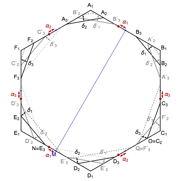
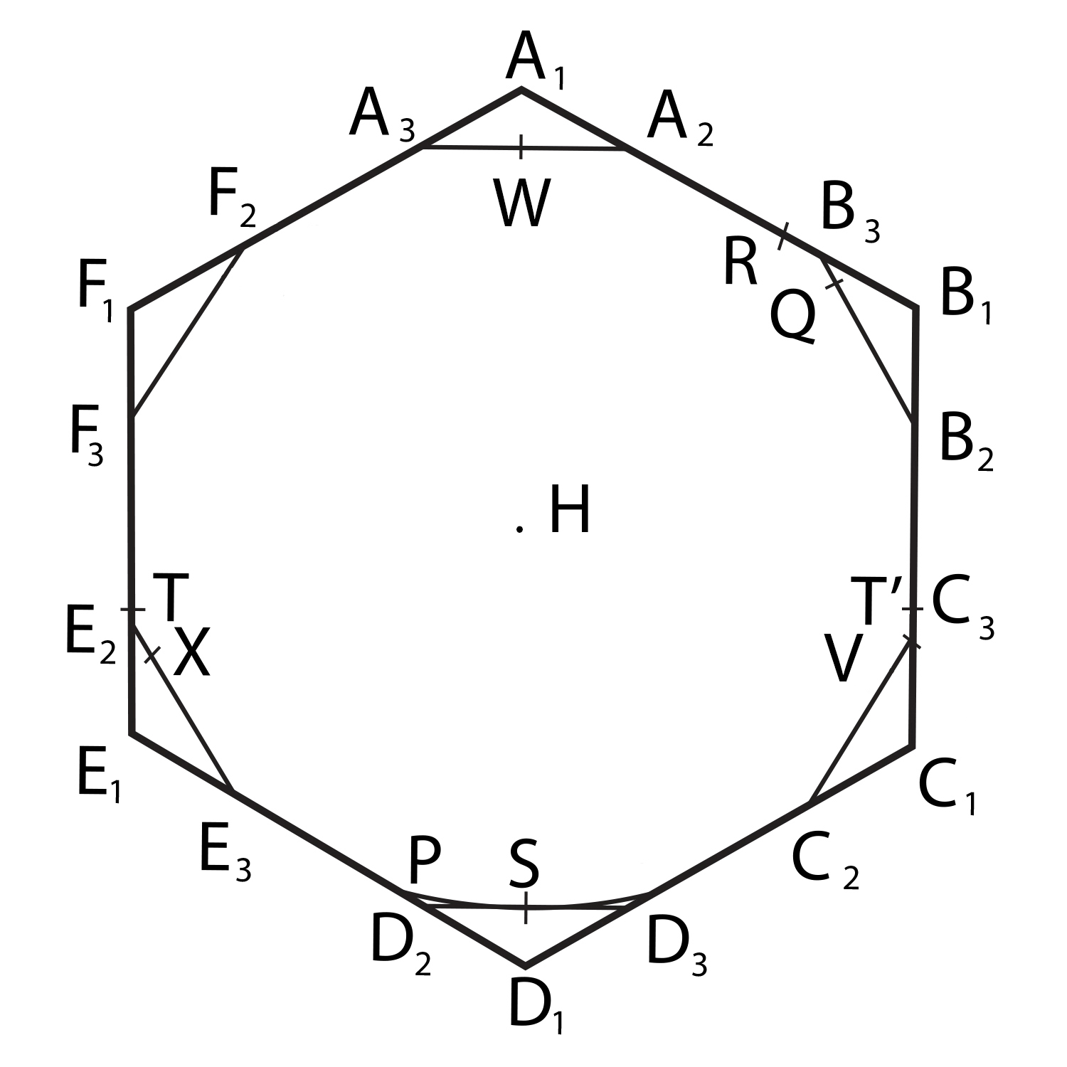
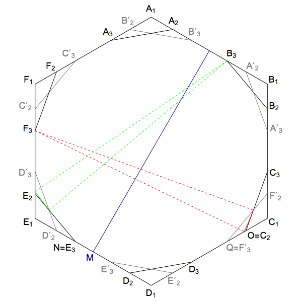
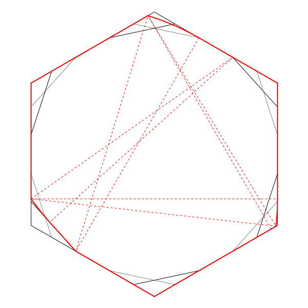
Any set SS of constant width 1 touches each side of a regular hexagon of width 1 at precisely one point. Each point of contact determines the one on the opposite side as well, so there is only a 3-parameter space of contact points; call the parameters α,β,γ\alpha, \beta, \gamma. Naively, 3 of the points can lie anywhere on their sides of the hexagon, but there’s an additional constraint that no pair of points can be separated by a distance greater than 1, which turns out to confine any pair of the three parameters to a certain intersection of ellipses.

Now, the set SS must lie inside the intersection of the six disks of radius 1 centred on the contact points; if we call that intersection of disks D(α,β,γ)D(\alpha, \beta, \gamma), then the union of D(α,β,γ)D(\alpha, \beta, \gamma) over the entire parameter space will give a universal covering. I haven’t checked, but I think that’s probably the entire hexagon.

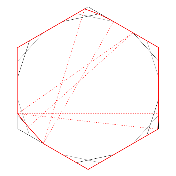
However, we can do a bit better than that quite easily: the 12-element symmetry group of the hexagon acts on the parameter space of 3-tuples (α,β,γ)(\alpha, \beta, \gamma), and there’s a natural partition of the parameter space into fundamental domains of that action. So the union of D(α,β,γ)D(\alpha, \beta, \gamma) over a single fundamental domain should also be a universal covering, once you take into account the possibility of applying the symmetries of the hexagon to the set you want to cover, in order to bring the contact points into the fundamental domain.

And the resulting set (which could probably be described analytically quite easily, but so far I’ve only constructed numerically) has an area of about 0.85.

But there might be some clever way to improve it …

Posted by: Greg Egan on February 12, 2015 11:47 AM | Permalink | Reply to this

Re: Can a Computer Solve Lebesgue’s Universal Covering Problem?

To bring the construction above a bit closer to the computability question, suppose we supplement the parameter space with 6n6n more parameters, describing the radial distance from the origin of the perimeter of the set SS we want covered, along each ray of a symmetrical 6n6n-pointed star. Again, there are constraints on the parameters due to the fact that the diameter of SS is 1, and if we take the intersection D(α,β,γ,r 1,...,r 6n)D(\alpha, \beta, \gamma, r_1, ..., r_{6n}) of the 6n+66n+6 unit disks centred at all of the points on the perimeter of SS that are fixed by the choice of parameters, then any such SS will be a subset of D(α,β,γ,r 1,...,r 6n)D(\alpha, \beta, \gamma, r_1, ..., r_{6n}).

Again the symmetries of the hexagon will act on the parameter space, and we can take the convex hull C nC_n of all the sets D(α,β,γ,r 1,...,r 6n)D(\alpha, \beta, \gamma, r_1, ..., r_{6n}) as the parameters range over a single fundamental domain of that action.

Each C nC_n will be a convex subset of the hexagon, so by the Blaschke selection theorem the sequence will at least contain a subsequence that converges to a convex set CC.

Posted by: Greg Egan on February 12, 2015 11:31 PM | Permalink | Reply to this

Re: Can a Computer Solve Lebesgue’s Universal Covering Problem?

A few things I should have made explicit about the construction described above:

The sequence of sets C nC_n will satisfy C n+1C nC_{n+1}\subseteq C_n, since adding parameters just introduces more constraints on the previous ones, and makes D(α,β,γ,r 1,...,r 6(n+1))D(\alpha, \beta, \gamma, r_1, ..., r_{6(n+1)}) the intersection of even more disks. So the sequence of areas of the C nC_n will be non-increasing.

It would be straightforward to write a program to explicitly construct any C nC_n as the set bounded by a finite number of arcs of algebraic curves (my hunch is quadratic curves, though that might be optimistic). By “straightforward” I mean I could probably actually do it, though it wouldn’t be trivial.

Also, I don’t think it should be too hard to prove that the limiting set CC of this sequence C nC_n is a subset of any universal covering that is a subset of the regular hexagon of width 1.

Posted by: Greg Egan on February 13, 2015 2:56 AM | Permalink | Reply to this

Re: Can a Computer Solve Lebesgue’s Universal Covering Problem?

I’m having a bit of trouble understanding your description of the set C nC_n, maybe because the description seems to invoke a specific set SS of constant width 1, but the set C nC_n is supposed to cover any such set SS. I’m pretty sure I’m just being slow-witted; you must be invoking SS merely to prove C nC_n really works, but I’m having trouble seeing what the set C nC_n really is.

Posted by: John Baez on February 13, 2015 7:20 AM | Permalink | Reply to this

Re: Can a Computer Solve Lebesgue’s Universal Covering Problem?

John wrote:

I’m having a bit of trouble understanding your description of the set C nC_n

OK, sorry, I’ll try to make this clearer!

Suppose WW is the collection of subsets of 2\mathbb{R}^2 of constant width 1. For any SWS \in W, I think the following things are true:

• There is a way to translate and rotate SS so that it becomes a subset of our favourite regular hexagon of width 1 centred at the origin, HH. That bit is just the fact that HH is a universal covering. So we might as well assume, wlog, that SS has already been translated and rotated in such a fashion, and that WW consists only of subsets of HH.

• Any SS will make contact with the perimeter of HH at six points, one on each edge. But these points come in pairs that lie at equal distances along opposite edges, so there are really only three parameters needed to describe all the possibilities there: say α,β,γ\alpha, \beta, \gamma.

• To get a further handle on the shape of any given SS, we can list the radial distances r ir_i from the origin to the perimeter of SS along 6n6n rays that form a symmetrical 6n6n-pointed star that is preserved by all the symmetries of HH.

• For a given choice of the parameters α,β,γ,r 1,...,r 6n\alpha, \beta, \gamma, r_1, ..., r_{6n}, there will still be uncountably many different sets that share them. Let’s give this subset of WW the name W(α,β,γ,r 1,...,r 6n)W(\alpha, \beta, \gamma, r_1, ..., r_{6n}). And what we can say about every SW(α,β,γ,r 1,...,r 6n)S \in W(\alpha, \beta, \gamma, r_1, ..., r_{6n}) is that it must be a subset of:

D(α,β,γ,r 1,...,r 6n)= pP(α,β,γ,r 1,...,r 6n)D(p,1)D(\alpha, \beta, \gamma, r_1, ..., r_{6n}) = \cap_{p\in P(\alpha, \beta, \gamma, r_1, ..., r_{6n})} D(p,1)

where D(p,1)D(p,1) is a unit disk centred on the point pp, and P(α,β,γ,r 1,...,r 6n)P(\alpha, \beta, \gamma, r_1, ..., r_{6n}) is a set of 6n+66n+6 points that lie at particular locations on the edges of HH, and on the 6n6n-pointed star. Since every SS is of diameter 1, every SS must be contained within any unit disk centred on any point it contains, and any SW(α,β,γ,r 1,...,r 6n)S \in W(\alpha, \beta, \gamma, r_1, ..., r_{6n}) contains the same 6n+66n+6 points, and hence must be a subset of D(α,β,γ,r 1,...,r 6n)D(\alpha, \beta, \gamma, r_1, ..., r_{6n}).

Now, the parameters α,β,γ,r 1,...,r 6n\alpha, \beta, \gamma, r_1, ..., r_{6n} will be subject to certain constraints, because they can never take on values such that two points in P(α,β,γ,r 1,...,r 6n)P(\alpha, \beta, \gamma, r_1, ..., r_{6n}) are separated by a distance greater than 1. Let’s call the appropriately constrained space of parameters Γ n\Gamma_n. Then:

W= α,β,γ,r 1,...,r 6nΓ nW(α,β,γ,r 1,...,r 6n)W = \cup_{\alpha, \beta, \gamma, r_1, ..., r_{6n} \in \Gamma_n} W(\alpha, \beta, \gamma, r_1, ..., r_{6n})

So, since any SW(α,β,γ,r 1,...,r 6n)S \in W(\alpha, \beta, \gamma, r_1, ..., r_{6n}) is covered by D(α,β,γ,r 1,...,r 6n)D(\alpha, \beta, \gamma, r_1, ..., r_{6n}), any SWS \in W will be covered by:

C n 0=convex hull of α,β,γ,r 1,...,r 6nΓ nD(α,β,γ,r 1,...,r 6n)C^0_n = \text{convex hull of } \cup_{\alpha, \beta, \gamma, r_1, ..., r_{6n} \in \Gamma_n} D(\alpha, \beta, \gamma, r_1, ..., r_{6n})

However, we can get a smaller covering by exploiting the symmetries of the hexagon!

The symmetries of the hexagon, D 6D_6, will act on the parameter space Γ n\Gamma_n in a fairly simple way, by exchanging edges of the hexagon and rays in the star. If we take a single fundamental domain for that action, call it Γ n (1)\Gamma^{(1)}_n, then we will have:

W (1)= α,β,γ,r 1,...,r 6nΓ n (1)W(α,β,γ,r 1,...,r 6n)W^{(1)} = \cup_{\alpha, \beta, \gamma, r_1, ..., r_{6n} \in \Gamma^{(1)}_n} W(\alpha, \beta, \gamma, r_1, ..., r_{6n})

where W (1)W^{(1)} is a subset of WW from which all of WW can be recovered by applying elements of D 6D_6. Equally, any SWS \in W will be mapped into W (1)W^{(1)} by some element of D 6D_6.

In other words, if we have any SWS \in W, we can rotate and/or reflect it with an element of D 6D_6 to get an isometric copy that lies in W (1)W^{(1)}, and so we don’t need to use the full range of parameters in Γ n\Gamma_n in order to cover it, we can make do with the smaller set, Γ n (1)\Gamma^{(1)}_n. So we define:

C n=convex hull of α,β,γ,r 1,...,r 6nΓ n (1)D(α,β,γ,r 1,...,r 6n)C_n = \text{convex hull of } \cup_{\alpha, \beta, \gamma, r_1, ..., r_{6n} \in \Gamma^{(1)}_n} D(\alpha, \beta, \gamma, r_1, ..., r_{6n})

C nC_n is a universal covering, because given any set SS of constant width 1 we can first translate and rotate it to become a subset of HH, and then we can rotate or reflect it to be a member of W (1)W^{(1)}. That is, we can ensure that the parameters that describe the points where this isometric copy of SS intersects the edges of HH and the rays of the 6n6n-pointed star belong to Γ n (1)\Gamma^{(1)}_n, and hence that SS is covered by one of the D(α,β,γ,r 1,...,r 6n)D(\alpha, \beta, \gamma, r_1, ..., r_{6n}) whose union makes up C nC_n.

Posted by: Greg Egan on February 13, 2015 9:21 AM | Permalink | Reply to this

Re: Can a Computer Solve Lebesgue’s Universal Covering Problem?

Okay, I think I get it now. I can see why you wanted to speak more informally and efficiently: all those formulas are a bit of a drag. But they got me over my confusion.

I guess I can’t tell if your sequence of sets C nC_n will converge to the minimum-area universal cover. It would be very nice to have an algorithm that was guaranteed to do that. I bet with more thought, maybe a lot more, one could get such an algorithm that’s not absurdly slow.

(My blog article is secretly a sketch of such an algorithm and proof that it works… but I bet it would be absurdly slow.)

Without such a guarantee, I guess you just have to run the algorithm and see how it does.

If it does well, I suspect most of the ‘excitement’ will occur near a few of the rays, in the sense that the radii r ir_i will turn out to do something predictable except near those rays. This at least seems to be the story of universal covers so far.

If so, you could then perhaps go in and pick formulas for most of the r ir_i, and space the rays more closely near the ‘exciting’ areas and have your algorithm spend most of its time on those.

But I’m getting ahead of myself… or yourself…

Posted by: John Baez on February 13, 2015 6:06 PM | Permalink | Reply to this

Re: Can a Computer Solve Lebesgue’s Universal Covering Problem?

John wrote:

I guess I can’t tell if your sequence of sets C nC_n will converge to the minimum-area universal cover.

There are three main obstacles I can see to proving that the C nC_n will converge to the minimum-area cover.

The first is the question of whether the minimum-area cover is a subset of the regular hexagon. That seems very likely. Do you know if anyone’s proved it?

The second is the question of whether you need to exploit further rotations or reflections that are not symmetries of the hexagon, in order to minimise the area of the cover. I’ve assumed that WW consists of sets of constant width 1 that have already been translated and rotated in order to fit inside the hexagon HH … but then I’ve assumed that any subsequent rotations or reflections must be symmetries of the hexagon. It seems possible, but it’s not obvious to me, that this is OK: that once you’ve exploited the full Euclidean isometry group to make an arbitrary set of constant width 1 into a subset of HH, there is nothing to be gained (in terms of minimising the area of the universal cover) by invoking the full isometry group again. Certainly, all the reductions to the hexagon rely on the ability to rotate or reflect the set to be covered using symmetries of the hexagon, rather than assuming any finer control. But it’s not obvious to me that there couldn’t be a set SS that fits in the hexagon, and will still fit in the hexagon after a certain rotation R(S)R(S) that isn’t a symmetry of either the hexagon or of SS itself, and that the possibility of covering R(S)SR(S) S rather than SS might allow for a reduction of the cover.

The third is the one that seems toughest to me. What I’m doing is, rather than covering all of WW, covering a subset of WW that contains one representative of each orbit of the symmetry group of the hexagon. That’s the subset I call W (1)W^{(1)}. But I’m choosing these representatives by making a “natural” choice of the fundamental domain of the action of the symmetry group on the parameter space. And maybe that’s not the right choice; maybe a different choice would give a smaller area.

I suppose the good thing about problem three is that it’s not necessarily fatal: the construction can always be modified to proceed with a different choice of fundamental domain. Intuitively, you’d expect that the fundamental domain in the parameter space that minimised the area of the convex hull of the union of all the sets in W (1)W^{(1)} would at least be a connected set … but hoping that it’s precisely a “Weyl chamber” (I’m putting that in quotes because I’m not sure it’s exactly the right term in this context, but it gives a good idea of what I’m using) might have been a tad optimistic. Still, it might be possible to figure out the optimal fundamental domain.

Anyway, what I really need to do is write a program to explicitly construct C nC_n, and see what kind of areas it yields. So far I’ve just numerically approximated C 0C_0, and as I mentioned its area is about 0.85. But as the 0th term in a guaranteed non-increasing series that’s not yet too discouraging.

Posted by: Greg Egan on February 13, 2015 11:31 PM | Permalink | Reply to this

Re: Can a Computer Solve Lebesgue’s Universal Covering Problem?

Greg wrote:

The first is the question of whether the minimum-area cover is a subset of the regular hexagon. That seems very likely. Do you know if anyone’s proved it?

No, I don’t. One might take a peek at Pál’s paper. I haven’t read it detail because it’s in German — a feeble excuse, because I know German; I just find it tiring. He’s the guy who proved the hexagon was a universal covering and showed you could cut off some corners and still get a universal covering. He might have tried to prove any universal covering lies in the hexagon.

Another place to look is the paper by Brass and Sharifi, who proved the best lower bound on the area of a universal covering. This is an engaging article, but I don’t see any result like the one you want.

So: this seems like a fun open problem.

Posted by: John Baez on February 14, 2015 1:12 AM | Permalink | Reply to this

Re: Can a Computer Solve Lebesgue’s Universal Covering Problem?

Greg wrote:

The first is the question of whether the minimum-area cover is a subset of the regular hexagon.

A word of warning: I don’t know if there is a unique universal covering of minimum area. So, you shouldn’t use the word ‘the’ here.

And here’s another word of warning…

In 1963, Eggleston found a universal covering that is minimal in a more general sense: no proper subset is a universal covering. Any universal covering with minimum area is minimal in this more general sense. However, the converse is not true! Eggleston’s minimal universal covering does not have the least possible area!

  • H. G. Eggleston, Minimal universal covers in E n,\mathrm{E}^n, Israel J. Math. 1 (1963), 149–155.

So, an algorithm could get ‘stuck in a false minimum’ if it proceeded by starting with a universal covering and continuing to chop pieces off!

(Hmm, I’m not sure if Eggleston was restricting attention to convex universal coverings, as we are doing.)

Posted by: John Baez on February 14, 2015 2:51 AM | Permalink | Reply to this

Re: Can a Computer Solve Lebesgue’s Universal Covering Problem?

Thanks for the warnings!

At this point I think the fastest way to learn something might be to charge ahead and try to construct the sequence of covers. It will probably go horribly wrong, but it should be easier to see why it goes wrong if I actually do it …

Posted by: Greg Egan on February 14, 2015 5:35 AM | Permalink | Reply to this

Re: Can a Computer Solve Lebesgue’s Universal Covering Problem?

The first is the question of whether the minimum-area cover is a subset of the regular hexagon. That seems very likely. Do you know if anyone’s proved it?

The numerical evidence supports it but it looks hard to prove.

It might be possible to make some progress with a related conjecture. From my annealing simulations I noticed that the following might by true:

The minimum-area cover for any set of curves of constant width one is a subset of a hexagon whose pairs of opposite sides are parallel and distance one apart.

This is still hard but there is some hope that it may be tractable. The first step is to prove that the minimum area cover for any set of curves of constant width one is a subset of a strip between two parallel lines of distance one apart. OK that one is easy so we are on our way. The second step would be to prove that the minimum-area cover for the set can be contained inside the intersection of two distinct strips of width one. I think that is doable but it would be good to see a rigorous proof written out. Probably this can be done using translations alone, no need for rotations or reflections. If you can get that far the last step would be to show that the minimum cover is contained in the intersection of three strips of width one. That would need to use the rotations and is going to be harder but it might yield to the same methods and just more hard work.

In fact if anyone wants to tackle a full proof they would be well advised to look first at the equivalent covering problem when only translations of shapes are allowed. A conjecture for this case would be that the cover is contained in a square. If that could be proved there would be hope that similar methods with much more detail would work for the regular hexagon when rotations are included.

Posted by: Philip Gibbs on February 14, 2015 9:31 AM | Permalink | Reply to this

Re: Can a Computer Solve Lebesgue’s Universal Covering Problem?

I got as far as an analytic construction for C 0C_0, but it seems clear to me now that my choice of parameters is not optimal, and that there’s no reason why the limit set of my sequence will do even as well as Pál’s cover.

So I’m going to try something a bit different, using parameters where Pál’s truncation occurs naturally from the choice of fundamental domain.

Posted by: Greg Egan on February 15, 2015 1:56 AM | Permalink | Reply to this

Re: Can a Computer Solve Lebesgue’s Universal Covering Problem?

Great! My warnings were not an attempt to discourage you or even make you slow down and think. I just wanted to give you all my limited knowledge about this problem.

Posted by: John Baez on February 15, 2015 9:36 PM | Permalink | Reply to this

Re: Can a Computer Solve Lebesgue’s Universal Covering Problem?

Here’s a framework that encompasses both the Pál truncation and the Gibbs-Bagdasaryan-Baez reduction.

Curve Parameters

We start with a regular hexagon of width 1. Then, as in the paper, take another copy of that hexagon rotated by an angle π6+σ\frac{\pi}{6}+\sigma, and a third hexagon that is the reflection of the rotated one in the blue line. Here, we only show the edges of the rotated and reflected hexagons when they are inside the original one; the edges of the reflected hexagon are in grey.

Given a curve of constant width 1 that has been translated and rotated to fit within the original hexagon, there are 9 parameters we measure. The three α i\alpha_i give the displacement from the centres of the hexagon’s edges to the points where the curve makes contact with those edges (shown as red dots). The three δ i\delta_i give the distance from the edges of the rotated hexagon to the lines that bound the curve most tightly that are parallel to those rotated edges. And the three δ i\delta'_i give the same distances for the reflected hexagon.

In the figure, the dashed lines drawn show what the bounds of a curve would be for a set of positive quantities for all the δ i\delta_i and δ i\delta'_i, in order to make the sign conventions clear, but all these variables can take on negative or positive values.

Now, in these terms Pál’s truncation amounts to claiming that we can always rotate the curve so that δ 10\delta_1 \ge 0 and δ 30\delta_3 \ge 0, leaving the triangles C 1C 2C 3C_1 C_2 C_3 and E 1E 2E 3E_1 E_2 E_3 empty, so we can remove them from the cover. We can think of this in terms of the action of the rotational symmetry group of the hexagon on the 3-dimensional space of triplets (δ 1,δ 2,δ 3)(\delta_1, \delta_2, \delta_3). Is there are fundamental domain of that action that meets Pál’s condition? There is:

F 1={(δ 1,δ 2,δ 3)|δ 10δ 30δ 1+δ 20δ 2+δ 30}F_1 = \{(\delta_1, \delta_2, \delta_3) | \delta_1 \ge 0 \wedge \delta_3 \ge 0 \wedge \delta_1+\delta_2 \ge 0 \wedge \delta_2+\delta_3 \ge 0\}

Any point in (δ 1,δ 2,δ 3)(\delta_1, \delta_2, \delta_3)-space will be mapped into F 1F_1 by some element of the hexagon’s rotational symmetry group. So we can always meet Pál’s condition.

For the Gibbs-Bagdasaryan-Baez condition, we need to go up to the full symmetry group of the hexagon, including reflections, and the full 9-parameter space. This condition adds to Pál’s the requirement that whenever δ 10\delta'_1 \ge 0 and δ 30\delta'_3 \ge 0, we have α 10\alpha_1 \le 0, in order to remove certain regions from the cover.

And again, there is a fundamental domain that satisfies this condition. I won’t write it down, because I haven’t been able to find one that can be described concisely; the best one I have is a union of 26 convex regions.

Now, of course these fundamental domains must exist, because their existence is just a restatement of the fact that the curves can always be rotated and/or reflected to meet the required conditions. But having these fundamental domains allows us to describe a sequence of covers whose areas will be bounded above by Pál’s area in the first case, or the Gibbs-Bagdasaryan-Baez area in the second case. I described the general idea earlier for a different parameter set, but with this improved choice of parameters we get a useful upper bound on the areas. With the current 9 parameters, we would impose the constraints that the red points of contact can’t lie outside the dashed lines of the curve’s bounds in various directions, or be separated from each other by a distance greater than 1, and then we would take the convex hull of the union, over all constrained parameters lying within the fundamental domain, of the intersection of the six unit disks centred on the red dots.

To refine things a little more, we could add six more parameters, pinning down the exact locations of the curve’s 12 points of contact with the dashed lines parallel to the rotated and reflected hexagon edges. In that case we would be taking intersections of 18 disks. And then the whole thing could be generalised to work with nn different rotated hexagons and their reflections, giving an infinite sequence of covers. The fundamental domains won’t change (in effect, we will just take their Cartesian product with the full space of all the extra parameters), but each set of additional parameters will impose additional constraints.

Of course, all I know so far is that the areas of these covers are bounded above by the Gibbs-Bagdasaryan-Baez area, and it might yet turn out that their areas are all simply equal to it; I haven’t shown that it’s possible to achieve any reduction at all! So it’s going to take some more work to answer that.

Posted by: Greg Egan on February 20, 2015 11:05 AM | Permalink | Reply to this

Re: Can a Computer Solve Lebesgue’s Universal Covering Problem?

As far as I can tell from some numerical investigations of the simplest case, the construction I discussed here merely reproduces the Gibbs-Bagdasaryan-Baez cover. The fact that I use a fundamental domain in the parameter space that is a proper subset of the set of parameters meeting the conditions discussed in the paper ends up making no difference.

Posted by: Greg Egan on February 26, 2015 10:04 AM | Permalink | Reply to this

Re: Can a Computer Solve Lebesgue’s Universal Covering Problem?

That’s interesting! I doubt we’ve found the optimal universal covering, but it sounds like you’re saying it’s the optimal one of some fairly natural class.

Posted by: John Baez on February 26, 2015 3:53 PM | Permalink | Reply to this

Re: Can a Computer Solve Lebesgue’s Universal Covering Problem?

Greg, I have already been able to progress some way beyond the cover in our paper so it is interesting to see how your approach matches up to mine. In our paper we looked at three cases which depend on the signs of the deltas in your picture.

To go further it is useful to consider all possible cases for the signs of the six deltas. Since two have to be positive that makes 16 cases. In fact only ten are distinct under reflections and rotations. I wonder if you could apply your methods to each case individually and then look for ways to amalgamate them.

I could post some pictures of the ten cases if it helps but what is the best way to post pictures here?

Posted by: Philip Gibbs on March 3, 2015 7:30 PM | Permalink | Reply to this

Re: Can a Computer Solve Lebesgue’s Universal Covering Problem?

It’s easy to post pictures in comments here using html. For example,

<img width = "300" src = "http://math.ucr.edu/home/baez/mathematical/lebesgue_universal_covering_hansen_modified.jpg" alt = "">

produces

The only annoying thing is that the system here uses a strict implementation of html so you’ll get an error message if you leave out the

alt = ""

part, which is designed to show some text if the image fails to display.

If you can’t put the pictures on a website to link to them, you can just send them to me and I’ll put them on my website. But I think you have a website!

Posted by: John Baez on March 3, 2015 9:09 PM | Permalink | Reply to this

Re: Can a Computer Solve Lebesgue’s Universal Covering Problem?

Wow, that sounds good! I’m busy grading homeworks and such, so I still haven’t gotten up the energy to carefully check your proof. But Philip Gibbs has a heuristic computer calculation pointing toward a value of

0.84408 0.84408

so there may be a couple more ‘large’ reductions left to make, shaving off an area of up to 3×10 53 \times 10^{-5}. I hope he tells us how breaking things into cases has helped him in his own recent work on this problem; I hear he’s pretty busy for the next couple weeks, but I’ll wait patiently for news.

Posted by: John Baez on March 4, 2015 1:42 AM | Permalink | Reply to this

Re: Can a Computer Solve Lebesgue’s Universal Covering Problem?

If you fix the sign of any single one of the six delta parameters in this diagram:

Curve parameters

… then that restricts the region that a curve of constant width 1 inscribed in the hexagon can occupy, to something isometric to this:

Curve of fixed delta sign

In that image I’ve fixed δ 10\delta_1 \ge 0, but you can get all the other signs and all the other deltas by rotating and or reflecting the same set.

There are three arcs on the boundary here, not just two! The one up the top is the Sprague reduction, the one on the left is the one I argued for here, and the third one, on the right, arises for essentially the same reason as the Sprague reduction: it’s due to the restriction of the point of contact of the curve of constant width to just part of one of the hexagon edges, because of the truncated corner.

Now in this particular case, you can say “so what?” about the third arc, because it lies inside a corner that’s going to be chopped off entirely. But for a general choice of a delta parameter and a sign, that’s not going to be the case, so this third arc need not generally be irrelevant.

I haven’t figured out all the consequences of this, but I’ll see how far I get trying to follow through Philip’s suggestion to break everything down by the signs of the deltas, intersect the sets associated with that choice of signs (imposing the extra restriction α 10\alpha_1 \le 0 when δ 10\delta'_1 \ge 0 and δ 30\delta'_3 \ge 0), and then take the convex hull of the union of all those intersections.

Posted by: Greg Egan on March 4, 2015 8:28 AM | Permalink | Reply to this

Re: Can a Computer Solve Lebesgue’s Universal Covering Problem?

Greg, it is good to see you working on this with some fresh ideas.

I think the whole covering problem now splits into two main parts. There is good evidence from the computational work I did that the optimum universal cover is a subset of a regular hexagon with two corners removed using the rotated hexagon as described in our paper (lets call it a slanted Pal cover) So part 1 is to prove that conjecture and for now that looks like a hard problem. Part 2 is to find the smallest universal cover with area a(σ)a(\sigma) that is a subset of a slanted Pal cover for a fixed slant angle σ\sigma. If both parts can be solved then the solution to the complete Lebesgue Universal Covering Problem is found just by taking the minimum of a(σ)a(\sigma)

In our paper we showed how to set an upper bound on a(σ)a(\sigma) for some range of σ\sigma. There is certainly room for improving this because our aim was to make the proof as simple as possible rather than getting the best bound. It is also possible to set lower bounds for this function simply because many curves of constant width fit into the slanted Pal cover in a unique way (e.g. the Reuleaux triangle and the circle to start with) Nothing has been said about this lower bound yet. My hunch is that this second part of the problem is quite tractable and in reach with some collaborative effort. Perhaps it would make a fun polymath problem.

Posted by: Philip Gibbs on February 22, 2015 8:11 AM | Permalink | Reply to this

Re: Can a Computer Solve Lebesgue’s Universal Covering Problem?

I thought that with all the people reading this blog who like constructive mathematics, there would be 50 comments by now. But maybe the language of ‘computable’ mathematics is sufficiently different from that of constructive mathematics that it seems off-putting? (Or maybe my post, where I was thinking out loud about a rather technical issue, was not well crafted to lure people into a discussion.)

Anyway, to me the great ‘miracle’ is the Blaschke selection theorem, which says that the space 𝒞\mathcal{C} of convex subsets of some ball in n\mathbb{R}^n, with its Hausdorff metric, is compact. A quick proof is here:

This means that searching through all these convex subsets, which seems initially like a hopeless task, is not so bad if we’re trying to find the maximum value of some continuous function

f:𝒞 f : \mathcal{C} \to \mathbb{R}

The function must be bounded and attain a maximum. What I’m wanting is an effective — that is a computable — version of this result. For this I think it’s enough for ff to be sequentially computable and computably uniformly continuous, and for 𝒞\mathcal{C} to be computably compact — as defined in my blog article.

I just noticed that kind of result could give a rigorous version of Philip Gibbs’ calculation of the number aa using simulated annealing. He took a bunch of convex shapes in the plane with diameter 1 and wiggled them around trying to find the convex set of least area that contained all of them. One problem with this strategy is that he couldn’t tell if he’d considered enough shapes to draw a conclusion about all such shapes.

However, if the space of convex shapes of diameter 1 is computably compact, we can find for any ϵ\epsilon a finite list of such shapes x ix_i such that any such shape has Hausdorff distance ϵ\le \epsilon from one of these shapes. And then I think we’ll know that any convex set that you can fit all these shapes x ix_i into will almost hold every shape of diameter 1. Here almost means that they may poke out a distance at most ϵ\epsilon. And this should be a big step toward rigorously computing the number aa.

Posted by: John Baez on February 12, 2015 4:48 PM | Permalink | Reply to this

Re: Can a Computer Solve Lebesgue’s Universal Covering Problem?

I wonder whether people don’t comment because there’s something wrong with the RSS feed and they haven’t actually seen this post yet?

I use the Café’s “comments” feed in Thunderbird to stay up to date with what’s happening here. Since I hadn’t seen any comments in a while, I’ve been wondering what was going on and noticed that I had missed some fascinating posts such as this one! So at least for me, the “comments” feed is currently not working.

Posted by: Tobias Fritz on February 17, 2015 6:05 PM | Permalink | Reply to this

Re: Can a Computer Solve Lebesgue’s Universal Covering Problem?

The RSS comments feed is working fine for me (although there was a blip a little while ago). I just don’t have much to contribute; I’m not that plugged into the computation side of constructive math. Although my general impression is that computational constructivity seems to approach things in a rather different way, so I wouldn’t be sure how to translate your programme into that language anyway: rather than defining something and then asking whether it’s computable, in order to even claim that it exists you have to define it in a computable way.

Posted by: Mike Shulman on February 17, 2015 8:05 PM | Permalink | Reply to this

Re: Can a Computer Solve Lebesgue’s Universal Covering Problem?

Hmm, I never use an RSS feed so I hadn’t noticed this. Thanks for mentioning it! I’ll inform the authorities.

I was really hoping, not that this post would get a lot of people working on Lebesgue’s universal covering problem, but that it would start a discussion of computable analysis, like the conditions under which the minimum value of a continuous function on a compact set is actually computable. There must be a big literature on this.

(Also the location of the minimum, but that seems harder, since there are cases where it’s very hard to tell which of two local minima is the ‘winner’.)

Posted by: John Baez on February 17, 2015 8:13 PM | Permalink | Reply to this

Re: Can a Computer Solve Lebesgue’s Universal Covering Problem?

Thanks! It’s back for me as well.

Posted by: Tobias Fritz on February 20, 2015 12:29 PM | Permalink | Reply to this

Re: Can a Computer Solve Lebesgue’s Universal Covering Problem?

I'm only reading this now, but I noticed that your definition of computable compactness only makes the space totally bounded; it also has to be complete to be compact.

Posted by: Toby Bartels on October 9, 2018 11:54 PM | Permalink | Reply to this

Re: Can a Computer Solve Lebesgue’s Universal Covering Problem?

Here’s a possible slight strengthening of “computability structure”: ask that the countable dense subset X iX_i is computably dense; that is, ask that there be a computable function HH such that {X i|i<H(n)} \{ X_i | i \lt H(n)\} is a 1n\frac{1}{n}-net. Until someone tells me this is already called something else (or follows from something more natural), I’ll call it “computably generated”.

I initially hoped this would follow from something else natural, (e.g. asking that the identity function should be computable), but I’m starting to despair. For example, I shouldn’t be surprised if there were shufflings of \mathbb{Q} supported on (say) the unit interval, and listed the rationals in [0,1][0,1] in such a clumpy way that you’d have to wait for a busy-beaver to finish to get a net of desired fineness.

There are definitely compact metric spaces that can’t be computably generated; For instance, let Θ\Theta be your favourite busy beaver function; then there’s a fine ultrametric on n{jΘ(n)}] \prod_n \{ j \leq \Theta (n) \} ] d(x,y)=11+min{j|x jy j} d(x,y) = \frac{1}{1 + min \{ j | x_j \neq y_j \} } but any 12+k\frac{1}{2+k}-net must have size much larger than Θ(k)\Theta(k). ((Of course, it’s more than possible that we don’t even have a computability structure on this space)).

Anyways, the point of asking for computable generation is that, for a computable-uniformly-continuous function ff, it should then be possible to compute a finite ε\varepsilon-net that covers each preimage f 1[pq±δ] f^{-1} [ \frac{p}{q} \pm \delta ] , and contained in f 1]pq±2δ[f^{-1} ] \frac{p}{q}\pm 2\delta [ .

Posted by: Jesse C. McKeown on February 18, 2015 12:13 AM | Permalink | Reply to this

Re: Can a Computer Solve Lebesgue’s Universal Covering Problem?

Well, I think I’ve convinced myself of the comforting proposition that the identity map is always computable, given an (ordinary) computability structure. Don’t know where this leaves computably generated vs. computable-structured and somehow compact.

Posted by: Jesse C. McKeown on February 23, 2015 4:00 AM | Permalink | Reply to this

Re: Can a Computer Solve Lebesgue’s Universal Covering Problem?

Yes, I’m pretty darn sure that computable metric spaces (separable metric spaces with computability structure) and computable functions between them form a category… so the identity function is computable, and composites of computable functions are computable.

Posted by: John Baez on February 23, 2015 7:56 AM | Permalink | Reply to this

Re: Can a Computer Solve Lebesgue’s Universal Covering Problem?

Philip, I’m not sure that my approach here leads anywhere useful. So far all I’ve seen is that going to the trouble of shrinking the parameter space to a fundamental domain of the symmetry group can turn out to make no difference at all!

In the mean time, I think I’ve found a simple and rigorously provable reduction of the cover from the paper:

Conjectured Reduction

I claim that you can remove the area between the red arc (part of a circle centred on F 3F_3) and the two straight edges of the original cover that this arc intersects, C 3C 2C_3 C_2 and C 2D 1C_2 D_1.

Why? Any curve of constant width 1 that fits inside the original cover must have a pair of points on its boundary that lie on two lines, parallel to the line segments F 2F 3F_2 F_3 and C 2C 3C_2 C_3, and are a distance of 1 apart. The rightmost point of this pair must lie to the left of C 2C 3C_2 C_3, since the whole of triangle C has been removed from the cover, and hence the leftmost point of the pair must lie to the left of F 3F 2F_3 F_2.

That means the curve must contain a point in the triangle F. And because the curve has diameter 1, it cannot contain any point whose distance from triangle F is greater than 1. But the region outside the red arc contains only points that are at a greater distance than 1 from any point in triangle F.

Now, crucially, I believe this reduction should be perfectly compatible with Reduction 3 in your paper, where in Case (3) you consider curves that don’t enter the reflected triangles E’ or C’. A mirror-image version of the argument I just gave means that any curve meeting those conditions can’t enter the reflection of the region I’ve just excluded, and hence you can safely reflect such curves without them entering the excluded region. So Reduction 3 still goes through without a hitch.

And all of this argument can be repeated with the area outside the green arc. Together, this leads to a reduction of about 6×10 76 \times 10^{-7}, and brings the upper bound on the cover area down to 0.8441147. And there’s at least one further (very tiny) reduction, since the arc that was originally centred at O in the original cover can also be shifted a small distance along the edge to the point where the red arc meets the edge.

The best way to post pictures here is just to use an HTML img tag referring to a file that you’ve uploaded elsewhere. Or for a large number of images you could just give a link.

Posted by: Greg Egan on March 5, 2015 5:21 PM | Permalink | Reply to this

Re: Can a Computer Solve Lebesgue’s Universal Covering Problem?

I claimed that there’s “at least one further (very tiny) reduction”, since the arc that was centred at O in the original cover can have its centre shifted a small distance along the edge C 2D 1C_2 D_1 to the point where the red arc meets that edge.

This turns out to be not so very tiny: it actually more than doubles the reduction, and puts an upper bound on the area of 0.8441140. This is despite it being necessary to increase the slant angle σ\sigma a tiny bit, in order to keep satisfying the condition that the angle WYQ is larger than a right angle.

Posted by: Greg Egan on March 5, 2015 5:23 PM | Permalink | Reply to this

Re: Can a Computer Solve Lebesgue’s Universal Covering Problem?

If you fix the sign of any single one of the six delta parameters in this diagram:

Curve parameters

… then that restricts the region that a curve of constant width 1 inscribed in the hexagon can occupy, to something isometric to this:

Curve of fixed delta sign

In that image I’ve fixed δ 10\delta_1 \ge 0, but you can get all the other signs and all the other deltas by rotating and or reflecting the same set.

There are three arcs on the boundary here, not just two! The one up the top is the Sprague reduction, the one on the left is the one I argued for here, and the third one, on the right, arises for essentially the same reason as the Sprague reduction: it’s due to the restriction of the point of contact of the curve of constant width to just part of one of the hexagon edges, because of the truncated corner.

Now in this particular case, you can say “so what?” about the third arc, because it lies inside a corner that’s going to be chopped off entirely. But for a general choice of a delta parameter and a sign, that’s not going to be the case, so this third arc need not generally be irrelevant.

I haven’t figured out all the consequences of this, but I’ll see how far I get trying to follow through Philip’s suggestion to break everything down by the signs of the deltas, intersect the sets associated with that choice of signs (imposing the extra restriction α 10\alpha_1 \le 0 when δ 10\delta'_1 \ge 0 and δ 30\delta'_3 \ge 0), and then take the convex hull of the union of all those intersections.

Posted by: Greg Egan on March 5, 2015 5:25 PM | Permalink | Reply to this

Re: Can a Computer Solve Lebesgue’s Universal Covering Problem?

Ah, we can even go one better, and remove the regions outside four arcs, not three!

Curve of fixed delta sign

This incorporates a second-order effect of a previous truncation: the restriction of the contact point along the top-left edge of the hexagon in turn restricts the contact point along the bottom-right edge, giving us another arc.

And all of this is a flow-on effect of truncating the original bottom-left corner.

Posted by: Greg Egan on March 5, 2015 5:26 PM | Permalink | Reply to this

Re: Can a Computer Solve Lebesgue’s Universal Covering Problem?

Greg, you have made a lot of progress. You are right that you can remove the area outside the arc centred on F 3F_3 and use that to improve the area removed around AA. You can also remove the area outside the arc centred on B 3B_3 shown on your diagrams, and there is a third area outside an arc centred on C 3C_3 which you must have noticed.

These reductions were already included in my paper http://vixra.org/abs/1401.0219 but the calculations there may not all be accurate. In the joint paper we wanted a simpler clearer proof with no errors so we did not include these reductions. It is good that you have rediscovered them. You are now ready to move onto the next level!

Below are the ten cases that need to be considered distinguished by the signs of the deltas. The red regions show where a curve of constant width does not enter in each case. Triangles EE and CC are always removed. Every such curve can fit into one of these cases but there are lines of reflection that allow the curves to be transformed. We have to find the best rules for when to reflect (or sometimes rotate) to make a subcover for each case. The union of all ten subcovers will then be a full universal cover.

Each case is a logical puzzle and some are more difficult than others. My best solution used hints from the numerical simulations that more area can be removed near AA and near E 2E_2 (see figure 26 in the paper) and the area of the best cover I have is 0.844093595. I dont know if it is the best possible but as I said earlier there is also scope for setting lower limits assuming a slanted covering.

Posted by: Philip Gibbs on March 5, 2015 5:29 PM | Permalink | Reply to this

Re: Can a Computer Solve Lebesgue’s Universal Covering Problem?

Philip wrote here:

… the area of the best cover I have is 0.844093595

Using what ought to be an equivalent approach, the best cover I find has an area of 0.844112132640. This is puzzling, because unless I’ve made a conceptual error or a programming error, this ought to be a lower bound for all covers that can be built simply by choosing signs for the δ\delta and α\alpha parameters.

So at this point I’m not sure if we’re intending to describe exactly the same set, and the discrepancy in areas is due to floating point round-off error, or if we’ve reached different conclusions about the smallest set of this kind that is a universal cover.

To try to resolve this, I’ll describe my calculations in some detail. Philip, please bear with me as I repeat a lot of things that you already know, but I want to try to give an account that’s reasonably self-contained, in case any interested bystander feels like checking it for errors of logic or geometrical reasoning. (It’s probably too much to hope that any third party will leap in and try to reproduce the actual numerical calculations.)

We’re considering curves of constant width 1 that have been translated and rotated to fit inside a regular hexagon of width 1. For each such curve, we can measure six parameters:

Curve Parameters

The parameters α 1,α 2,α 3\alpha_1, \alpha_2, \alpha_3 measure the distance from the centres of the hexagon’s edges to the points where the curve makes contact with those edges (the red points on the diagram, though the diagram does not include any actual curve). There are only 3 such parameters, rather than 6, because if the curve makes contact with edge EE at a certain point PP, it must make contact with the edge parallel to EE at the unique point that is a distance of 1 from PP.

The δ\delta parameters relate to two copies of the original hexagon: one that has been rotated counter-clockwise by an angle of π6+σ\frac{\pi}{6}+\sigma (where for the moment σ\sigma is a free parameter), and another that is the reflection of that rotated one, in any of the original hexagon’s axes of symmetry. (In the diagram, I’ve used reflection in the blue line to map certain named features to their primed reflections, following the notation in the joint paper. Philip uses a different notation in his diagrams here, giving triangles the same letter, primed, when they intersect, which is probably more sensible … but in any case, in what follows I’ll avoid triangle names and just refer to the δ\delta parameters on the diagram.)

The parameters δ 1,δ 2,δ 3\delta_1, \delta_2, \delta_3 measure the perpendicular distance from the edges of the rotated hexagon to the two supporting lines for the curve (the dashed lines on the diagram) that are parallel to each pair of those rotated edges. Similarly, the parameters δ 1,δ 2,δ 3\delta'_1, \delta'_2, \delta'_3 measure the same thing for the rotated-and-reflected hexagon.

Now, suppose we’re handed a particular curve of constant width 1, placed inside the hexagon. We measure its nine parameters, which might initially have any of 512 possible 9-tuples of signs. (We’ll be sloppy and just treat 0 as positive by fiat.) However, by rotating and/or reflecting the curve using any of the 12 isometries of the hexagon, we can change the 9 signs and guarantee that they always end up in a smaller set of possibilities than the initial 512.

The advantage of this is seen most dramatically in the choice that was made by Pál (see here, and the linked paper for details), who showed that you can always rotate a curve so that δ 1>0\delta_1 \gt 0 and δ 3>0\delta_3 \gt 0. If you do that, then the curve will always fit inside a hexagon that has had two corners cut off: the regions where δ 1<0\delta_1 \lt 0 and δ 3<0\delta_3 \lt 0.

Let’s take it as self-evident that it will always be good to retain Pál’s choice of restrictions (if we didn’t, we’d end up merely making minor tweaks to the full hexagon, having lost the huge reduction of the cover’s area that comes from cutting off two corners). We then have just 128 9-tuples of signs for the parameters, and we can ask what further restrictions are possible.

The 12-element isometry group of the hexagon acts on the set of 9-tuples of signs by moving them on 52 orbits. Some of these orbits will, of course, take the 9-tuples outside the set of 128 defined by Pál’s restriction, so we simply focus on the portions of each orbit that continue to obey that restriction.

If we do this, it turns out that 14 of the 128 9-tuples of signs have just one 9-tuple in their restricted orbit. This means we’re stuck with them. The others fall into 38 orbits of various sizes: 19 of size 2, 2 of size 3, 16 of size 4 and 1 of size 6, which in principle means we have:

2 19×3 2×4 16×6=1.21597189939003392×10 172^{19} \times 3^2 \times 4^{16} \times 6 = 1.21597189939003392 \times 10^{17}

choices for a selection of 52 9-tuples of signs into which we could rotate any curve. Fortunately, it turns out that we don’t need to check anything remotely connected to this terrifying number.

To go further, we need to talk about the specific subsets of the hexagon that will cover any curve that has a restriction on the sign of one of its parameters. If we restrict the sign of a δ\delta parameter, we get a restricted cover like this:

Cover for choice of delta sign

If we restrict the sign of an α\alpha parameter, we get a restricted cover like this:

Cover for choice of alpha sign

In these images, arcs of circles of radius 1 that form part of the boundary are marked by drawing dashed lines from their endpoints to the centre of the circle of which they are part.

For the δ\delta-sign restricted cover, it’s obvious that we can cut one corner off the hexagon, but why are there arcs on parts of the boundary? The reason is that if you draw a supporting line L CL_C for the cover CC at any point on its boundary, then a curve of constant width 1 that sits inside the cover will itself have two supporting lines, L 1L_1 and L 2L_2, a distance of 1 apart, that are parallel to L CL_C. The one closest to L CL_C must lie on the interior side of L CL_C, in order for the curve to be inside the cover; call that one L 1L_1. But this means that L 2L_2 must lie a distance of 1 or more away from L CL_C. It then follows that some point of the curve (the point that lies on L 2L_2) must lie in the subset of CC that is a distance of 1 or more from the line L CL_C; call that subset C 1C_1. But since the curve has diameter 1, no point of the curve can lie anywhere in CC that is a distance of more than 1 from C 1C_1.

For the δ\delta-sign restricted cover, putting a support line along the edge created by the truncation makes C 1C_1 into the triangle at the opposite corner of the hexagon. This restricts the cover to points that lie within a circle of radius 1 centred at one corner of that triangle. But as we move the support line around the shape, we get three other arcs as well.

Something similar happens with the α\alpha-sign restricted cover, except that rather than excising a two-dimensional region, we’ve omitted one half-edge of the hexagon by declaring that no curve can touch it. Putting a support line L CL_C along the opposite edge gives us a C 1C_1 that consists of the non-omitted half-edge, and no point of the curve can lie at a greater distance of 1 from that half-edge. Then as we move the support line around we get the other three arcs.

Depending on the particular parameter number and sign, the restricted covers will just be rotated and/or reflected versions of the two I’ve drawn above (though in the case of the δ\delta parameters, the covers will also depend on the value of σ\sigma that’s being used; in the diagrams above I’ve used a huge 12 degrees for the sake of clarity).

To restrict ourselves to any particular 9-tuple of signs, we take the intersections of the appropriate 9 individual restricted covers, one for each parameter. No curve with the nominated 9-tuple of signs for its 9 parameters will lie outside that intersection.

The final task, then, is to choose 52 such 9-tuples of signs, in a way that minimises the area of the convex hull of the union of all 52 9-fold-intersections of restricted covers. This will be a universal cover, because we have chosen one 9-tuple from each of the 52 orbits. Whatever original 9-tuple of signs we have for a curve – which could be anything in the full set of 512 possibilities – there will be some rotation and/or reflection of the hexagon that brings it to one of our chosen 52.

Now, the bad news was that there are, in principle:

2 19×3 2×4 16×6=1.21597189939003392×10 172^{19} \times 3^2 \times 4^{16} \times 6 = 1.21597189939003392 \times 10^{17}

ways to choose a 9-tuple on each orbit. The good news comes if we start by focusing on the 14 9-tuples where we have no choice, because there is only one element in the orbit (subject to the Pál restriction). We can take the 14 associated restricted covers and form the convex hull of their union; we will call this the “compulsory hull” because we have no choice, we must include it.

But the nice surprise that saves us from a combinatorial nightmare is this: if we take the convex hull of the union of this “compulsory hull” with each of the 12814=114128-14=114 restricted covers corresponding to the 9-tuples where we need to make a choice, it turns out that in every orbit but one, there is at least one 9-tuple whose restricted cover is already contained within the compulsory hull. Obviously, then, for those 52141=3752-14-1=37 orbits, we should choose one such 9-tuple … and it will make no difference at all to the final union which such 9-tuple we choose.

That leaves the single orbit with no restricted cover inside the compulsory hull. And this orbit only contains two 9-tuples.

Now, my claim that certain restricted covers were subsets of the compulsory hull is something I checked across a range of angles of interest for σ\sigma, from 0.5 degrees to 1.5 degrees. So anywhere in that range the same logic applies: we will get the minimal area for the final cover by choosing between the two 9-tuples in the sole orbit where we have a meaningful choice to make. So we compute the areas of the final cover for each of these two choices for a range of angles. It turns out that one choice is better across the whole range, and for an angle of σ=1.0424\sigma = 1.0424 degrees, the smaller cover has a total area of 0.844112132640. It looks like this:

Universal cover with area 0.844112132640

And in fact, this set is exactly the same as the set that’s obtained by making the choices in the joint paper: δ 1>0,δ 3>0\delta_1 \gt 0, \delta_3 \gt 0 and when δ 1>0\delta'_1 \gt 0 and δ 3>0\delta'_3 \gt 0 we choose α 1<0\alpha_1 \lt 0. None of the finer-grained decisions about the other four parameters end up offering any further reduction. The only reason the area is slightly less than the area in the joint paper (0.8441153) is that (a) in that paper, not all the regions-outside-arcs that could be removed by restricting the sign of each parameter were removed, and (b) the cover here uses a value for σ\sigma low enough to cause a certain angle to be less than a right angle, which in the joint paper was ruled out (I guess because it would have complicated the proof).

Philip, your ten diagrams show a representative from each of the ten orbits of the action of the symmetry group on the 6-tuples of δ\delta parameter signs. But in order to compare covers, could you state explicitly what restrictions you’re imposing on the α\alpha parameters in each of these ten cases, and what value you’re using for σ\sigma for your best cover? That will tell me if we’re talking about the same sets.

Also, if there are further reductions you’re exploiting beyond those shown in the two diagrams I give above, for a restriction on a delta sign and a restriction on an alpha sign, can you explain what they are? If not, we ought to be working with exactly the same sets and doing the same things with them, so we ought to end up agreeing, up to any differences in floating point round-off.

Posted by: Greg Egan on March 7, 2015 10:59 PM | Permalink | Reply to this

Re: Can a Computer Solve Lebesgue’s Universal Covering Problem?

Greg, one quick comment before I work through what you have done. Although I am selecting cases on only the sign of the deltas, I am not using just the sign of the alphas to decide when to reflect. That was the case for our paper but to go further I have been using more complex criteria to decide when to reflect the curves so as to be able to remove more pieces.

Posted by: Philip Gibbs on March 8, 2015 6:10 PM | Permalink | Reply to this

Re: Can a Computer Solve Lebesgue’s Universal Covering Problem?

Greg, I can give you a bit more detail so you can see how to move forward.

Let’s concentrate on the triangle EEE'-E in my pictures, near the point E 2E_2 in yours. You already know that a small part of this can be removed using arcs centred on C 3C_3 and B 3B_3 but let’s try and remove some more. This can be done case by case. In cases where the triangle is coloured red in my diagrams the whole triangle is clear so no need to worry about those cases. That leaves CEADC'E'A D', CEDAC'E'D A', FEAAF'E'AA', FEADF'E'A D' and FEDAF'E'D A'.

For the first two cases the sign of α 3\alpha_3 can be used to remove the part of EEE'-E which is outside an arc centred on the midpoint of B 1C 1B_1C_1

For cases FEAAF'E'A A' and FEDAF'E'D A' you might be tempted to use the sign of α 2\alpha_2 but it does not help. Instead you use the hexagon rotated at an angle of π6\frac{\pi}{6} and introduce yet another δ\delta for the edges near EE and BB. Using the axis of reflection you can then choose the sign of that new δ\delta and that allows about half of the triangle EEE'-E to be removed for these two cases.

The remaining case is FEADF'E'A D'. This is the hardest one. I’ll come back to that later :-)

When these are all considered together there is some area that is removed in every case so this (or rather its convex hull) can be removed from the final cover.

Posted by: Philip Gibbs on March 8, 2015 9:49 PM | Permalink | Reply to this

Re: Can a Computer Solve Lebesgue’s Universal Covering Problem?

Philip, so far all I’ve been able to determine is that the signs of the 12 parameters we’ve discussed (the 9 original ones plus 3 related to a hexagon rotated by exactly π6\frac{\pi}{6}) are not sufficient to deal with the case FEADF' E' A D'.

If you don’t have time to describe your construction in detail, can you at least describe the basic principle? Does it involve a new set of parameters whose signs are used in the same manner as the previous ones? Or does it involve some finer-grained dissection of the existing parameter space?

Posted by: Greg Egan on March 10, 2015 1:34 PM | Permalink | Reply to this

Re: Can a Computer Solve Lebesgue’s Universal Covering Problem?

Sorry this is brief but you have to reflect so that the curve cuts or touches the line F 2F 3F_2F_3 somewhere outside FF'. This then sets a constraint on α 3\alpha_3. Hope I got that right I don’t have my notes to hand.

I hope to have more time next week.

Posted by: Philip Gibbs on March 10, 2015 2:40 PM | Permalink | Reply to this

Re: Can a Computer Solve Lebesgue’s Universal Covering Problem?

Philip, I’ll have to wait until you have some free time to explain your reduced cover in detail, because I remain stumped by the FEADF' E' A D' case!

For example:

Reuleaux 7-gon for F'E'A D'

The green curve is the border of a Reuleaux 7-gon. The red curve is the restricted cover for the FEADF' E' A D' case.

The green curve belongs to the FEADF' E' A D' case, with small positive values for δ 1,δ 2,δ 3\delta_1, \delta_2, \delta_3 and small negative values for δ 1,δ 2,δ 3\delta'_1, \delta'_2, \delta'_3. It occupies a fraction 1ϵ1-\epsilon of the part of the reduced cover inside the triangle EEE'-E, where ϵ\epsilon can be made arbitrarily small (but not zero) by making the values of the δ\delta coefficients arbitrarily small (but retaining the necessary signs).

The green curve shares the reduced cover’s symmetry, reflection in the line F 1C 1F_1 C_1, so that reflection can’t clear any space in the triangle EEE'-E. All other symmetries of the hexagon take parts of the green curve into triangles C or E, violating the Pál condition.

Also, as far as I’m able to determine, there are no other isometries that position the green curve differently inside the hexagon.

So if any more of triangle EEE'-E is removed from the cover, how can this 7-gon be made to fit?

Posted by: Greg Egan on March 11, 2015 1:35 PM | Permalink | Reply to this

Re: Can a Computer Solve Lebesgue’s Universal Covering Problem?

Greg, that’s a good point. I believe the answer to this counterexample is that the argument only works for slant angles below some value σ 0\sigma_0.

Let’s call GG the point of intersection of the line segments F 3F 2F_3F_2 and C 2C 3{C'}_2{C'_3} in your notation. There is an angle σ 0\sigma_0 for which the distance from GG to C 3C_3 is exactly one (what is this angle?). At all other angles it is greater than one.

In the FEADF'E' A D' case the curve must intersect or touch the V-shaped line F 3GC 3F_3G{C'}_3. Now reflect the curve if necessary so that it intersects F 3GF_3G

For slant angles less than σ 0\sigma_0 all points on the segment F 3GF_3G are at a distance greater than one from C 3C_3 This is not true for larger angles. There is therefore a constraint on α 3\alpha_3. In fact the curve must touch the side B 1C 1B_1C_1 above the point on the side which is at a distance one from GG. We can remove points outside the arc centred on that point near E 2E_2

I don’t have a note to hand of the optimal slant angle but it is about 2 degrees I think.

Posted by: Philip Gibbs on March 11, 2015 6:46 PM | Permalink | Reply to this

Re: Can a Computer Solve Lebesgue’s Universal Covering Problem?

Thanks, Philip! That’s extremely helpful.

BTW, the angle σ 0\sigma_0 turns out to be precisely π18\frac{\pi}{18}, i.e. 10 degrees. I’ve been using 12 degrees when visualising these examples, for the sake of clarity, but I didn’t think carefully enough about the qualitative changes that choice imposed.

Posted by: Greg Egan on March 12, 2015 12:18 AM | Permalink | Reply to this

Re: Can a Computer Solve Lebesgue’s Universal Covering Problem?

Indeed, it does change qualitatively. Earlier I said it would be interesting to calculate a(σ)a(\sigma) the area of the smallest cover contained in a hexagon with two corners removed at a slant angle σ\sigma. The minimum might be the best cover and it is certainly an upper bound.

However, this gets harder for large σ\sigma. the largest σ\sigma is 30 degree at which point we arrive back at a complete hexagon. So a(π6)a(\frac{\pi}{6}) is the area of the best cover that can fit inside a hexagon, which is no bigger than a(σ)a(\sigma) for any other σ\sigma. I think that a(σ)a(\sigma) is not continuous at that point though.

Now that you know what happens near EE you might want to consider what extra area can be removed near AA.

Posted by: Philip Gibbs on March 12, 2015 1:54 PM | Permalink | Reply to this

Re: Can a Computer Solve Lebesgue’s Universal Covering Problem?

OK, I’ve just realised that there’s at least one potential problem with my analysis here. I was assuming that we could take the restricted covers we get by choosing signs for each parameter, individually, and then simply intersect them to get the restricted cover for curves where we have chosen signs for multiple parameters.

And of course those intersections are covers for the appropriately restricted curves … but they’re not as small as they could be! The various excisions we made from the original sets by running a support line around them won’t necessarily include all the excisions we can make from the intersection. For example:

Further reductions to intersections of reduced covers

The set with an outline in red shows the intersection of the nine sets we get when we individually choose the signs of each of the nine parameters to be positive. But if we draw a support line along the lower right-hand truncation that we’ve made in order that δ 3>0\delta_3 \gt 0, the line parallel to it a distance of 1 away (the green line in the upper left) defines a portion of the original cover (the small region inside the red set that lies to the left of that green line), within which there must be some point of any curve that fits in the cover. So any part of the cover at a distance greater than 1 from that region (i.e. any part outside the two green arcs) is superfluous.

So I’ll need to go back and redo my whole analysis, taking care to remove as much as possible from each of these sets corresponding to a 9-tuple of signs.

Posted by: Greg Egan on March 8, 2015 5:37 AM | Permalink | Reply to this

Re: Can a Computer Solve Lebesgue’s Universal Covering Problem?

Having used the supporting line method to trim excess regions from the restricted covers for the 9-tuples of parameter signs, I can still only bring the area of the final cover down from my previous value of 0.844112132640 to 0.844112120469, a reduction of about 1.2×10 81.2 \times 10^{-8}.

Some of the individual restricted covers can be trimmed by quite large amounts: up to an enormous 0.00195152. But the “compulsory hull” of all the restricted covers associated with 9-tuples of sign choices that need to be included in the final cover is only reduced by 1.2×10 81.2 \times 10^{-8}, hence the final result.

Posted by: Greg Egan on March 8, 2015 5:01 PM | Permalink | Reply to this

Re: Can a Computer Solve Lebesgue’s Universal Covering Problem?

It took me nearly three years to get round to it but here finally is a write-up of how I get the improved upper bound of 0.844093595

An Upper Bound for Lebesgue’s Universal Covering Problem

Posted by: Philip Gibbs on January 22, 2018 10:52 PM | Permalink | Reply to this

Re: Can a Computer Solve Lebesgue’s Universal Covering Problem?

Hello Greg Egan,

I find your idea of computable function over convex shapes very interesting. I had an idea for such a function and I would be very interested on your feedback. My background is in engineering so I may lack mathematical rigor and tackle the problem more on the algorithmic side.
I emphasize on three assumptions that I cannot prove, hopefully there are sound arguments for those.

Hope you find it interesting

Posted by: SergeKireev on December 12, 2018 10:18 PM | Permalink | Reply to this

Re: Can a Computer Solve Lebesgue’s Universal Covering Problem?

Here it goes:

I. Simulation procedure

Two preliminary (unproven) assumptions:

*Every convex shape of diameter 1 is contained in a shape of constant width 1 (noted CWS)

*Every CWS can be approximated at an arbitrary precision by a CWS with a finite n number of “pinching points” (noted PP) For further information on PPs and an algorithm to construct CWS: http://cgm.cs.mcgill.ca/~athens/cs507/Projects/2001/BB/cs507/

So we focus on CWS with a finite n number of PPs

Trivially, every such shape has an odd number of PPs, and each of the points is at a distance 1 of exactly 2 other PPs, such as we can link them as an arbitrarily shaped star: http://cgm.cs.mcgill.ca/~athens/cs507/Projects/2001/BB/cs507/5.gif

The star we extract from the shape is a graph with exactly 1 cycle. n-3 consecutive angles (by walking the graph) formed at the vertices, entirely characterize the shape. Only n-3 is due to the fact that only N-1 points characterize the shape, as the last one is equidistant to PP1 and PPn-1 and closer to other PPs

So we can encode any shape with n PPs by a n-3 tuple of real numbers each belonging to [0, pi/3] (pi/3 because the only shape which can have a pi/3 angle is trivially the reuleux triangle)

Now for the simulation we just have to iterate with a sufficient precision on all possible tuples in lexical order.

II. Estimation of errors

Three types of errors:

  1. Sampling error Error due to sampling when iterating over tuples (missing shapes between chosen values)

  2. Left shapes error When having iterated through all shapes with number of PPs <= n, all shapes with PPs > n are left. How well were they approximated by the shapes we already iterated through?

  3. Approximation of minimal cover At each step we compute an approximation of a minimal cover for a set of shapes

III. Estimation of computation complexity and optimisation proposals

1: Computation complexity To iterate through all shapes of n points with e precision on angles: (pi/3e)^(n-3) steps. At each step we calculate the minimal coverage by rotating and translating current shape relatively to the others (let’s suppose that this is a constant number of steps)

Which brings us to O((1/e)^n) steps for computing the cover of all shapes with number of PPs <= n

2: Parallel computation

*Unproven assumption (to challenge): The minimal coverage for a finite set of convex shapes has additive structure. For two shapes A and B, we define sum of A and B as the minimal coverage of A and B. We suppose that we have partial associativity: if we have a set S1 of shapes with area > A and another set S2 with area <= A we assume that sum(S1) + sum(S2) = sum(S1 union S2)

We can massively parallelize the computation as addition of independent set of shapes can be done on separate nodes and then aggregated.

I will try to make some simulations as I have most of the code to generate arbitrary shapes already. Keep you posted.

Posted by: SergeKireev on December 12, 2018 10:23 PM | Permalink | Reply to this

Post a New Comment