Re: The Modular Flow on the Space of Lattices
Here’s some stuff I wrote about certain aspects of this business:
May 20, 2006
This Week’s Finds in Mathematical Physics (Week 233)
On Tuesday I’m supposed to talk with Lee Smolin about an idea he’s
been working on with Fotini Markopoulou and Sundance Bilson-Thompson.
This idea relates the elementary particles in one generation of the
Standard Model to certain 3-strand framed braids:
1) Sundance O. Bilson-Thompson, A topological model of composite
preons, available as hep-ph/0503213.
2) Sundance O. Bilson-Thompson, Fotini Markopoulou, and Lee Smolin,
Quantum gravity and the Standard Model, hep-th/0603022.
It’s a very speculative idea: they’ve found some interesting relations,
but nobody knows if these are coincidental or not.
Luckily, one of my hobbies is collecting mysterious relationships between
basic mathematical objects and trying to figure out what’s going on.
So, I already happen to know a bunch of weird facts about 3-strand braids. I figure I’ll tell Smolin about this stuff. But if you don’t mind, I’ll
practice on you!
So, today I’ll try to tell a story connecting the 3-strand braid group,
the trefoil knot, rational tangles, the groups SL(2,Z) and PSL(2,Z),
conformal field theory, and Monstrous Moonshine.
I’ve talked about some of these things before, but now I’ll introduce
some new puzzle pieces, which come from two places:
3) Imre Tuba and Hans Wenzl, Representations of the braid group B3
and of SL(2,Z), available as math.RT/9912013.
4) Terry Gannon, The algebraic meaning of genus-zero, available as
math.NT/0512248.
You could call it "a tale of two groups".
On the one hand, the 3-strand braid group has generators
     |   |   |
      \ /    |
A  =   /     |
      / \    |
     |   |   |
and
     |   |   |
     |    \ /
B =  |     /
     |    / \
     |   |   |
and the only relation is
ABA = BAB
otherwise known as the "third Reidemeister move":
|   |  |         |  |   |
 \ /   |         |   \ /
  /    |         |    /
 / \   |         |   / \
|   \ /           \ /   |
|    /      =      /    |
|   / \           / \   |
 \ /   |         |   \ /
  /    |         |    /
 / \   |         |   / \
On other hand, the group SL(2,Z) consists of 2×2 integer matrices with determinant 1. It’s important in number theory, complex analysis,
string theory and other branches of pure mathematics. I’ve described
some of its charms in "week125", "week229" and elsewhere.
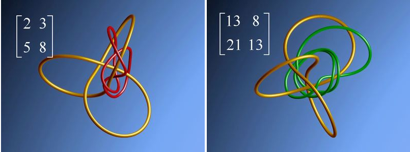
These groups look pretty different at first. But, there’s a
homomorphism from B3 onto SL(2,Z)! It goes like this:
        1   1
A |->
        0   1
        1   0
B |->
       -1   1
Both these matrices describe "shears" in the plane.
You may enjoy drawing these shears and visualizing the equation
ABA = BAB in these terms. I did.
I would like to understand this better… and here are some clues.
The center of B3 is generated by the element (AB)3.
This element corresponds to a "full twist". In other words, it’s
the braid you get by hanging 3 strings from the ceiling, grabbing
them all with one hand at the bottom, and giving them a full 360-degree
twist:
|   |  |
 \ /   |
  /    |       A
 / \   |
|   \ /
|    /         B
|   / \
 \ /   |
  /    |       A
 / \   |
|   \ /
|    /         B
|   / \
 \ /   |
  /    |       A
 / \   |
|   \ /
|    /         B
|   / \
|  |   |
This full twist gets sent to -1 in SL(2,Z):
             -1   0
(AB)^3 |->
              0  -1
So, the double twist gets sent to the identity:
             1   0
(AB)^6 |->
             0   1
In fact, Tuba and Wenzl say the double twist generates the
kernel of our homomorphism from B3 to SL(2,Z). So, SL(2,Z)
is isomorphic to the group of 3-strand braids modulo double twists!
This reminds me of spinors… since you have to twist an electron
around twice to get its wavefunction back to where it started. And indeed, SL(2,Z) is a subgroup of SL(2,C), which is the double cover of the Lorentz group. So, 3-strand braids indeed act on the state space of a spin-1/2 particle, with double twists acting
trivially!
(For more on this, check out Trautman’s work on "Pythagorean
spinors" in "week196".
There’s also a version where we use integers mod 7, described in
"week219".)
If instead we take 3-strand braids modulo full twists, we get the
so-called "modular group":
PSL(2,Z) = SL(2,Z)/{+-1}
Now, SL(2,Z) is famous for being the "mapping class group"
of the torus - that is, the group of orientation-preserving
diffeomorphisms, modulo diffeomorphisms connected to the identity.
Similary, PSL(2,Z) is famous for acting on the rational numbers
together with a point at infinity by means of fractional linear
transformations:
         az + b
z |->   -------
         cz + d
where a,b,c,d are integers and ad-bc = 1. The group PSL(2,Z) also
acts on certain 2-strand tangles called "rational tangles".
In "week229", I told a nice
story I heard from Michael Hutchings, explaining how these three facts
fit together in a neat package.
But now let’s combine those facts with the stuff I just said! Since
PSL(2,Z) acts on rational tangles, and there’s a homomorphism from
B3 to PSL(2,Z), 3-strand braids must act on rational
tangles. How does that go?
There’s an obvious guess, or two, or three, or four, but let’s just
work it out.
I just said that the 3-strand braid A gets mapped to this shear:
        1   1
A |->
        0   1
In "week229" I said what this
shear does to a rational tangle. It gives it a 180 degree twist at
the bottom, like this:
  |   |                |   |
  |   |                |   |
  |   |                |   |
 -------              -------
 |  T  |   |---->     |  T  |
 -------              -------
  |   |                 \ /
  |   |                  /
  |   |                 / \
Next, Tuba and Wenzl point out that
                  0   1
ABA = BAB |->
                 -1   0
which is a quarter turn. From "week229" you can see how this quarter turn
acts on a rational tangle:
  |   |                       |     |
  |   |              ____     |     |
  |   |             /     \   |     |
 -------           |     -------    |
 |  T  |   |---->  |     |  T  |    |
 -------           |     -------    |
  |   |            |      |   \____/
  |   |            |      |
  |   |            |      |
It gives it a quarter turn!
From these facts, we can figure out what the braid B does to a
rational tangle. So, let me do the calculation.
Scribble, scribble, curse and scribble…. Eureka!
Since we know what A does, and what ABA does, we can figure out
what B must do. But, to make the answer look cute, I needed a
sneaky fact about rational tangles, which is that A also acts
like this:
  |   |                 \ /
  |   |                  /
  |   |                 / \
 -------              -------
 |  T  |   |---->     |  T  |
 -------              -------
  |   |                |   |
  |   |                |   |
  |   |                |   |
This is proved in Goldman and Kauffman’s paper cited in "week228".
With the help of this, I can show B acts like this:
  |   |              |          |
  |   |              |   ___    |
  |   |              |  /   \   |
 -------             | /    -------
 |  T  |   |---->     \     |  T  |
 -------             / \    -------
  |   |             |   \___/   |
  |   |             |           |
  |   |             |           |
And this is great! It means our action of 3-strand braids on
rational tangles is really easy to describe. Just take your tangle
and let the upper left strand dangle down:
           |
   ____    |
  /    \   |
 |    -------
 |    |  T  |
 |    -------
 |     |   |
 |     |   |
 |     |   |
To let a 3-strand braid act on this, just attach it to the bottom of
the picture!
(That’s why there were four obvious guesses about this would work: one can easily imagine four variations on this trick, depending on
which strand is the "odd man out" - here it’s the upper right. It’s just a matter of convention which we use, but my conventions give this.)
In fact, even the group of 4-strand braids acts on rational tangles in
an obvious way, but the 3-strand braid group is enough for now.
Let me summarize.
The 3-strand braid group B3 acts on rational tangles
in an obvious way. The subgroup that acts trivially is precisely the
center of B3, generated by the full twist.
Using stuff from "week229",
it follows that the quotient of B3 by its center acts
on the projectivized rational homology of the torus. We thus get a topological explanation
of why B3 mod its center is PSL(2,Z).
But there’s more.
For starters, the 3-strand braid group is also the fundamental group of
S3 minus the trefoil knot!
And, S3 minus the trefoil knot is secretly the same as
SL(2,R)/SL(2,Z)!
In fact, Terry Gannon writes that the 3-strand braid group can be
regarded as "the universal central extension of the modular
group, and the universal symmetry of its modular forms". I’m not
completely sure what that means, but here’s part of what it
means.
Just as PSL(2,C) is the Lorentz group in 4d spacetime, PSL(2,R) is the
Lorentz group in 3d spacetime. This group has a double cover SL(2,R),
which shows up when you study spinors. But, it also has a universal
cover, which shows up when you study anyons. The universal cover has
infinitely many sheets. And up in this universal cover, sitting over
the subgroup SL(2,Z), we get… the 3-strand braid group!
In math jargon, we have this commutative diagram where the
rows are short exact sequences:
    1 ----> Z -----> B^3 -------> SL(2,Z) ----> 1
            |        |             |
            |        |             |
            v        v             v
    1 ----> Z ---> SL(2,R)~ ---> SL(2,R) ----> 1
Here SL(2,R)~ is the universal cover of SL(2,R).
Since π1(SL(2,R)) = Z, this is a Z-fold cover.
You can describe this cover explicitly using the Maslov index,
which is a formula that actually computes an integer for any loop
in SL(2,R), or indeed any symplectic group.
But anyway, fiddling around with this diagram and the long exact
sequence of homotopy groups for a fibration, you can show that indeed:
π1(SL(2,R)/SL(2,Z)) = B3.
This also follows from the fact that
SL(2,R)/SL(2,Z) looks like S3 minus a trefoil.
Gannon believes that number theorists should think about all this stuff,
since he thinks it’s lurking behind that weird network of ideas called
Monstrous Moonshine (see "week66").
And here’s the basic reason why. I’ll try to get this right….
Any rational conformal field theory has a "chiral algebra" A which
acts
on the left-moving states. Mathematicians call this sort of thing a
"vertex operator algebra". A representation of this on some vector
space V is a space of states for the circle in some "sector" of our
theory. Let’s pick some state v in V. Then we can define a
"one-point function" where we take a Riemann surface with little
disk cut out and insert this state on the boundary. This is a number,
essentially the amplitude for a string in the give state to evolve like
this Riemann surface says.
In fact, instead of chopping out a little disk it’s nice to just
remove a point - a "puncture", they call it. But, we get an ambiguous
answer unless we pick coordinates at this point, or in the lingo of
complex analysis, a choice of "uniforming parameter". Then our
one-point function becomes a function on the moduli space of Riemann
surfaces equipped with a puncture and a choice of uniformizing parameter.
If we didn’t have this uniformizing parameter to worry about, we’d
just have the moduli space of tori equipped with a marked point,
which is nothing but the usual moduli space of elliptic curves,
H/PSL(2,Z)
where H is the complex upper halfplane. Then our one-point function
would have nice transformation properties under PSL(2,Z).
But, with this uniformizing parameter to worry about, our one-point
function only has nice transformation properties under B3. This
is somehow supposed to be related to how B3 is the "universal
central extension" of PSL(2,Z): in conformal field theory, all sorts
of naive symmetries hold only up to a phase, so you have to replace
various groups by central extensions thereof… and here that’s what’s
happening to PSL(2,Z)!
That last paragraph was pretty vague. If I’m going to understand this
better, either someone has to help me or I’ve got to read something
like this:
5) Yongchang Zhu, Modular invariance of characters of vertex operator algebras,
J. Amer. Math. Soc 9 (1996), 237-302. Also available at
http://www.ams.org/jams/1996-9-01/S0894-0347-96-00182-8/home.html
But I shouldn’t need any conformal field theory to see how the moduli
space of punctured tori with uniformizing parameter is related to the
3-strand braid group! I bet this moduli space is X/B3 for
some space X, or something like that. There’s something simple at the
bottom of all this, I’m sure.
Addenda: Another relation between the trefoil and
the punctured torus: the trefoil has genus 1, meaning that
it bounds a torus minus a disc embedded in R3.
You can see this in the lecture "Genus and knot sum" in
this course on knot theory:
6) Brian Sanderson, The knot theory MA3F2 page,
http://www.maths.warwick.ac.uk/~bjs/MA3F2-page.html
This course also has material on rational tangles.
The fact that B3 is a central extension of
PSL(2,Z) by Z, and the quantum-mechanical interpretation of
a central extension in terms of phases, plays an important role
here:
7) R. Voituriez, Random walks on the braid group B3
and magnetic translations in hyperbolic geometry, Nucl. Phys. B621
(2002), 675-688. Also available as
http://arxiv.org/abs/math-ph/0103008.
Among other things, he points out that the homomorphism
B3 → SL(2,Z) described above is the "Burau
representation" of B3 evaluated at t = 1.
In general, the Burau representation of B3 is given
by:
        t   1
A |->
        0   1
        1   0
B |->
       -t   t
(Conventions differ, and this may not be the best, but it’s
the one he uses.) The Burau representation can also be used
to define a knot invariant called the Alexander polynomial.
I believe that with some work, one can use this to explain
why Conway could calculate the rational number associated to a
rational tangle in terms of the ratio of Alexander polynomials of two
links associated to it, called its "numerator" and
"denominator". In fact he computed this ratio of
polynomials and then evaluate it at a special value of t -
presumably the same special value we’re seeing here (modulo
differences in convention).
Another issue: I wrote
For starters, the 3-strand braid group is also the fundamental group of
S3 minus the trefoil knot!
And, S3 minus the trefoil knot is secretly the same as
SL(2,R)/SL(2,Z)!
The first one is pretty easy to see; you start with the "Wirtinger
presentation" of the fundamental group of S3 minus a
trefoil, and show by a fun little calculation that this isomorphic to the braid group on 3 strands. A more conceptual proof would be very nice, though. (See "week261" for such a proof - and much more on all this stuff.)
What about the second one? Why is S3 minus the trefoil knot
diffeomorphic to SL(2,R)/SL(2,Z)? Terry Gannon says so in his paper above, but doesn’t say why. Some people asked about this, and eventually some people found
some explanations. First of all, there’s a proof on page 84 of this book:
8) John Milnor, Introduction to Algebraic K-theory, Annals of Math.
Studies 72, Princeton U. Press, Princeton, New Jersey, 1971.
Milnor credits it to Quillen. Joe Christy summarizes it below. I
can’t tell if this proof is essentially the same as another sketched
below by Swiatoslaw Gal, which exhibits a diffeomorphism using
functions called the Eisenstein series g2 and
g3. They are probably quite similar arguments.
Joe Christy writes:
I wouldn’t be surprised if this was known to Seifert in the 30’s,
though I can’t lay my hands on Seifert & Threfall at the moment to
check. Likewise for Hirzebruch, Brieskorn, Pham & Milnor in the 60’s in
relation to singularities of complex hypersurfaces and exotic spheres.
When I was learning topology in the 80’s it was considered a warm up
case of Thurston’s Geometrization Program - the trefoil knot complement
has PSL(2,R) geometric structure.
In any case, peruse Milnor’s Annals of Math Studies for concrete
references. There is a (typically) elegant proof on p.84 of
"Introduction to Algebraic K-theory" [study 72], which Milnor credits
to Quillen. It contains the missing piece of John’s argument:
introducing the Weierstrass P-function and remarking that the
differential equation that it satisfies gives the diffeomorphism to
S3-trefoil as the boundary of the pair (discriminant of diff-eq,
C2 = (P,P’)-space).
This point of view grows out of some observations of Zariski, fleshed
out in "Singular Points of Complex Hypersurfaces" [study 61]. The
geometric viewpoint is made explicit in the paper "On the Brieskorn
Manifolds M(p,q,r)" in "Knots, Groups, and 3-manifolds" [study 84].
It is also related to the intermediate case between the classical
Platonic solids and John’s favorite Platonic surface - the
Klein quartic. By way of a hint, look to
relate the trefoil, qua torus knot, the seven-vertex triangulation of
the torus, and the dual hexagonal tiling of a (flat) Clifford torus in
S3.
Joe
Swiatoslaw Gal writes:
In fact the isomorphism is a part of the modular theory:
Looking for
f: GL(2,R)/SL(2,Z) → C2 - {x2=y3}
(there is an obvious action of R+ on both sides:
M |→ tM for M in GL(2,R),
x |→ t6 x, y |→ t4 y,
and the quotient is what we want).
GL(2,R)/SL(2,Z) is a space of lattices in C.
Such a lattice L has classical invariants
g2(L) = 60 sum_{z in L’} z-4,
and
g3(L) = 140 sum_{z in L’} z-6,
where L’=L-{0}
The modular theory asserts that:
1. For every pair (g2,g3) there exist a
lattice L such that g2(L) = g2 and
g3(L) = g3 provided that
g23 is not equal to
27g32.
2. Such a lattice is unique.
Best,
S. R. Gal
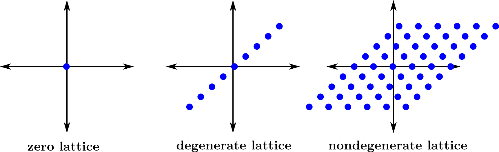
The quantity g23 - 27
g32 is called the "discriminant" of the
lattice L, and vanishes as the lattice squashes down to being
degenerate, i.e. a discrete subgroup of C with one rather than two
generators.
.")

Re: The Modular Flow on the Space of Lattices
That’s a very nice post Bruce.
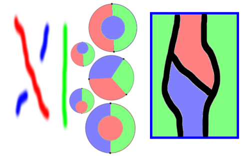
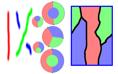
I first learnt about the space of non-degenerate lattices up-to-homothety being the complement of the trefoil from my friend and old office-mate Jacob Mostovoy.
He has a nice, short paper on how this space is related to subsets of the circle with at most three elements.