The n-Category Café

Simple functions on the line

Let’s begin in one dimension. Our aim is to define the integral $\int f \; d \chi$ for suitable functions $f\colon \mathbf{R} \to \mathbf{R}$.

Whatever we think Euler characteristic is, the Euler characteristic of a compact, nonempty interval $A$ should be $1$. So, writing $I_A$ for the indicator function (or characteristic function) of $A$, we should have

$$\int I_A \;d \chi = 1.$$

Since integration is supposed to be linear, this tells us how we must integrate any finite linear combination of indicator functions of compact nonempy intervals. I’ll call these simple functions on $\mathbf{R}$. So, for a simple function

$$f = \sum_{r = 1}^k c_r I_{A_r},$$

where each $A_r$ is a compact nonempty interval, we should have

$$\int f \;d \chi = \sum_{r = 1}^k c_r.$$

Do I hear you sigh? If you’ve seen this kind of thing before, you’ll recognize the standard problem: the definition isn’t obviously consistent, since $f$ can be expressed as a combination of indicator functions in multiple ways, and maybe these give multiple different values for the integral. In that case, you’ll also know that the standard solution, involving common refinements, is pretty tedious work.

Happily, we can avoid it. Here’s how. For a simple function $f$, put

$$J(f) = \sum_{x \in \mathbf{R}} (f(x) - f(x-))$$

where $f(x-)$ means $lim_{\varepsilon \to 0+} f(x - \varepsilon)$. This quantity $J(f)$ is well-defined, linear in $f$, and takes value $1$ when $f$ is the indicator function of a compact nonempty interval. So, $J(f) = \sum c_r$ whenever $f = \sum c_r I_{A_r}$. We therefore put

$$\int f \;d \chi = J(f),$$

and the consistency problem evaporates.

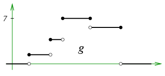
Let’s have some examples. What, for instance, is the integral against the Euler characteristic of this function?

The solid and empty circles indicate that $f(a) = f(b) = 0$. So

$$f = 3I_{(a, b)} = 3I_{[a, b]} - 3I_{[a, a]} - 3I_{[b, b]}$$

and

$$\int f \;d\chi = 3 - 3 - 3 = -3.$$

Since $f = 3I_{(a, b)}$, this tells us that we’re treating the Euler characteristic of the open interval $(a, b)$ as $-1$. That might strike you as wrong if you’re used to Euler characteristic being invariant under homotopy equivalence. But as James Propp pointed out long ago, there’s a tension between the requirement that Euler characteristic is homotopy-invariant and the requirement that it behaves like a finitely additive measure. You can’t have both at once. (See also John Baez’s excellent talk on the mysteries of counting.) Here we’re not worrying about homotopy invariance; we’re using what Propp would call ‘Euler measure’.

What about this function?

It’s not hard to see that $\int g \;d\chi = 7$, whatever the unlabelled values on the axes might happen to be. I chose the letter $J$ to stand for ‘jump’: $J(f) = \int f \;d\chi$ is the total vertical jump occurring at jump discontinuities from the left.

One more example: what is the integral against the Euler characteristic of the following function?

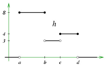
Here

$$h = 3 I_{[a, d]} + 5 I_{[a, b]} + I_{[c, d]},$$

so

$$\int h \;d\chi = 3 + 5 + 1 = 9$$

(regardless of the values of $a$, $b$, $c$ and $d$). Alternatively, you can calculate $\int h \;d\chi$ via the formula for $J(f)$, giving $8 + (4 - 3) = 9$ again.

More general functions on the line

Classical measure theory also involves things called ‘simple functions’ (with a different but analogous meaning). There, defining integration for simple functions is just a prelude to defining integration for a larger class of functions. Can we do something similar here, extending our integral to a larger class of functions?

We can. Indeed, the formula

$$\sum_{x \in \mathbf{R}} (f(x) - f(x-))$$

for $\int f \;d\chi$ immediately makes sense for more than just the simple functions.

But before we charge ahead and generalize, let’s correct the ugly asymmetry you see here. In everything so far, we could equally well have used the formula

$$\sum_{x \in \mathbf{R}} (f(x) - f(x+)).$$

It makes no difference: this is still equal to $\int f \;d\chi$ for simple functions $f$. Of course, it’s just as asymmetric. However, taking the average of the two formulas, we also have

$$\int f \;d\chi = \frac{1}{2} \sum_{x \in \mathbf{R}} \bigl[-f(x-) + 2f(x) - f(x+)\bigr].$$

This is now symmetric, and therefore more likely to give us a useful definition for more general functions $f$.

(Maybe you can see a hint of how curvature is going to enter the story: this looks like the expression $$f''(x) = \displaystyle\lim_{\varepsilon\to 0} \frac{f(x-\varepsilon) - 2f(x) + f(x+\varepsilon)}{\varepsilon^2}$$ for a second derivative, and second derivatives have something to do with curvature.)

So: let $f\colon \mathbf{R} \to \mathbf{R}$ be a function such that the limits $f(x-)$ and $f(x+)$ exist for all $x \in \mathbf{R}$, and are equal to $f(x)$ for all but finitely many $x \in \mathbf{R}$. In other words, $f$ is continuous except for a finite number of jump discontinuities. The integral against the Euler characteristic of such a function $f$ is defined by the formula above:

$$\int f \;d\chi = \frac{1}{2} \sum_{x \in \mathbf{R}} \bigl[ -f(x-) + 2f(x) - f(x+) \bigr].$$

Be warned: this has some properties that you might not expect of an integral. For instance, the integral of any continuous function is $0$, the integral of a function that is everywhere strictly positive can be strictly negative, and changing the value of a function at a single point can change the value of the integral. On the other hand, this integral has some interesting properties too, as we’ll see when we get to higher dimensions.

Simple functions in higher dimensions

Let’s now consider functions on $\mathbf{R}^n$, for $n \geq 1$. The role of intervals will be played by convex sets. For brevity, I’ll use ‘convex’ to mean ‘compact, nonempty and convex’.

A function $f\colon \mathbf{R}^n \to \mathbf{R}$ is simple if it can be expressed as a finite linear combination of indicator functions of convex sets. Again, we want to ‘define’

$$\int f \;d\chi = \sum_{r = 1}^k c_r$$

whenever $f = \sum_{r = 1}^k c_r I_{A_r}$ for some convex sets $A_r$, and again we might groan at the prospect of having to do those tedious consistency checks.

But once more, the jump functional $J$ comes to the rescue. I’ll explain in the case $n = 2$; the strategy for higher dimensions should be clear. Let $f\colon \mathbf{R}^2 \to \mathbf{R}$ be a simple function. For each $x \in \mathbf{R}$, the function

$$f(x, -)\colon \mathbf{R} \to \mathbf{R}$$

is simple, and so we can define a function $F\colon \mathbf{R} \to \mathbf{R}$ by $F(x) = J(f(x, -))$. This function $F$, too, is simple, so we get a real number $J(F)$. We define $J(f)$ to be this number: $J(f) = J(F)$.

Thus, we have defined $J(f)$ for every simple function $f$ on $\mathbf{R}^2$. It is linear in $f$, with $J(1_A) = 1$ whenever $A$ is convex. So just as in the one-dimensional case, $J(f) = \sum c_r$ when $f = \sum c_r I_{A_r}$. This solves the consistency problem, and $\int f \;d\chi = J(f)$.

I learned this from Chapter 5 of Klain and Rota’s Introduction to Geometric Probability (source of so many wonderful things). It is remarkably little effort, and is even based on a very standard technique: reducing a multivariable integral to a sequence of single-variable integrals. But it has an immediate nontrivial consequence: the definition of Euler characteristic for a large class of subsets of $\mathbf{R}^n$.

Indeed, call a subset $S$ of $\mathbf{R}^n$ polyconvex if it can be expressed as a finite union of convex sets. For example, any picture on a black and white television is polyconvex (assuming that each pixel is convex). And quite simply, we define

$$\chi(S) = \int I_S \;d\chi.$$

You can prove, as Klain and Rota do, that this coincides with the usual definition.

More general functions in higher dimensions, and curvature

The rough idea now is that given a function $f\colon \mathbf{R}^n \to \mathbf{R}$ whose discontinuities are no worse than those of a simple function, we should be able to define $\int f \;d\chi$ by repeating verbatim the definition for simple functions.

In the one-dimensional case, we first had to deal with the pesky problem that the formula

$$J(f) = \sum_{x \in \mathbf{R}} (f(x) - f(x-))$$

isn’t symmetric, so probably wouldn’t generalize well. To fix that, we considered the formula $\sum (f(x) - f(x+))$ obtained by reversing the orientation of the line, and then we averaged over the two orientations to get something symmetric.

In higher dimensions, the asymmetry problem can no longer be brushed aside with this algebraic flick of the wrist. In fact, some interesting geometry comes in here. This asymmetry issue, which looked like a nuisance distracting us from the main business, turns out to be exactly the reason why integration against the Euler characteristic is closely related to curvature.

Again I’ll stick to $n = 2$, leaving higher dimensions to your imagination.

In defining $J(f)$ for simple functions $f\colon \mathbf{R}^2 \to \mathbf{R}$, we used the standard coordinate system on $\mathbf{R}^2$. When $f$ is simple, the choice of basis does not affect the value of $J(f)$ (which is always equal to $\sum c_r$, if $f = \sum c_r I_{A_r}$). But for more general functions $f$, it certainly does make a difference. What we should do is consider all ordered orthonormal bases of $\mathbf{R}^2$, calculate $J(f)$ with respect to each basis, and define $\int f \;d\chi$ to be the average.

(You can see that this generalizes what we did for $\mathbf{R}^1$: there we took the average of two things, and there are two orthonormal bases of $\mathbf{R}^1$.)

I don’t want to make this post any longer by explaining exactly what, for instance, ‘average’ means. Nor will I say much about which functions $f$ this will be a reasonable definition for. Instead, I’ll focus on the geometric interpretation of $\int f \;d\chi$.

Let’s think about a function $f\colon \mathbf{R}^2 \to \mathbf{R}$ of the form $g \cdot I_A$, where $g$ is continuous and $A$ is convex. Thus, $f$ is supported on $A$ and continuous everywhere except perhaps on the boundary of $A$, where it might jump in value as it crosses the boundary. I’ve just been reading something that talks about functions `suffering a jump discontinuity’. The suffering of $f$ is limited to $\partial A$.

What is $\int f \;d\chi$? How can we understand it?

Well, $\int f \;d\chi$ is the average over all orthonormal bases of the quantity “$J(f)$ with respect to that basis”. So, take an orthonormal basis — a coordinate system — and let’s consider $J(f)$.

Recall that the definition of $J(f)$ was slicewise. For each $x \in \mathbf{R}$, we take the function $f(x, -)\colon \mathbf{R} \to \mathbf{R}$ and put $F(x) = J(f(x, -))$. In the picture, the value of $x$ shown is in the vertical shadow of $A$, so $F(x)$ is equal to $f(x, y)$.

Now since $f$ is continuous, $F$ is too, except that $F$ has a jump discontinuity at each end of the shadow. So, $J(F) = f(x_0, y_0)$. Finally, by definition, $J(f) = J(F)$, and so $J(f) = f(x_0, y_0)$.

So in the end, $J(f)$ is something really trivial:

$J(f)$ is the value of $f$ at the leftmost point of $A$

where ‘leftmost’ refers to the basis concerned. (I’m assuming for simplicity that the boundary of $A$ is smooth and contains no line segments. This isn’t crucial.)

But this isn’t the same as $\int f \;d\chi$. To get that, we have to average over all orthonormal bases of $\mathbf{R}^2$. That is, we slowly rotate our coordinate axes through $360^\circ$, at each moment recording the value of $f$ at the ‘leftmost’ point of $A$ (with respect to the current axes), then taking the mean. As we rotate, that leftmost point works itself around the whole boundary of $A$, never backtracking. And here’s the important thing:

It spends more time at some boundary points than others.

To see why, consider a convex set like this:

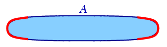
For almost all choices of axes, the leftmost point of $A$ will be in one of the red parts of the boundary. Only rarely will it be elsewhere.

So as we rotate the axes, the leftmost point with respect to the axes moves quickly over parts of the boundary with low curvature, and lingers where the curvature is high. We’d therefore imagine that $\int f \;d\chi$ would be the integral of $f$ over the boundary of $A$ with respect to some kind of curvature measure on $\partial A$.

This turns out to be true. In fact,

$$\int f \;d\chi = \int_{\partial A} f d\phi$$

where $\phi$ is the angle that the tangent makes with some fixed, arbitrarily chosen reference line:

This is good, but there’s another way to put it too. When we integrate along a curve, we usually do it with respect to the arclength measure, typically written as $d s$. And the rate of change of the angle $\phi$ per unit arclength is nothing but the classical curvature $\kappa$. That is, $\kappa = d\phi/d s$. Putting this together with the last equation, we get

$$\int f \;d\chi = \int_{\partial A} f\cdot\kappa \; d s.$$

So, the integral against the Euler characteristic of a function of this type is naturally expressed in terms of curvature.

You can go further down this track. If you know about intrinsic volumes, you can ask and answer the question: what does it mean to integrate against an intrinsic volume? You’ll see that each intrinsic volume corresponds to a different curvature measure; in $n$ dimensions, we get $n$ different curvature measures on the boundary of a convex set.

What I’d like to know is how much of this story is well-known. Curvature measures are extremely well-studied, and connections between curvature and Euler characteristic go back to the Gauss–Bonnet theorem at least. On the other hand, I’ve never heard anyone talking explicitly about integration against the Euler characteristic. Does anyone know where this stuff is written up?