Musings

David Lyth showed that a detectable signal in tensor modes implies a lower bound on the excursion, in field space, of the inflaton during inflation.

The power in tensor modes is directly related to the height of the inflaton potential,

In slow-roll inflation, $P_s$ is enhanced, relative to this

where $ϵ=\frac{1}{2}{M}_p^2{\left(\frac{V\prime }{V}\right)}^2$ is the slow-roll parameter. Combining (1) and (2),

where $d𝒩$ is the differential number of e-foldings. This gives the total field variation of the inflaton during inflation as $$\frac{\Delta \varphi }{M_p}=\frac{1}{\sqrt{8}}{\int }_0^{{𝒩}_{\text{end}}}\sqrt{r(𝒩)}d𝒩$$ where ${𝒩}_{\text{end}}\sim 60$.

$r(N)$ may vary considerably, from the beginning to the end of inflation. What we expect to be able to measure, however, is the ratio on CMB scales ($2<\ell \lesssim 100$, corresponding to $0<𝒩\lesssim 4$), so it behoves us to define an $${𝒩}_{\text{eff}}={\int }_0^{{𝒩}_{\text{end}}}\sqrt{r(N)/r_{\text{CMB}}}d𝒩$$ and write

After relating the logarithmic rate of change of $r$ to the scalar and tensor spectral indices¹

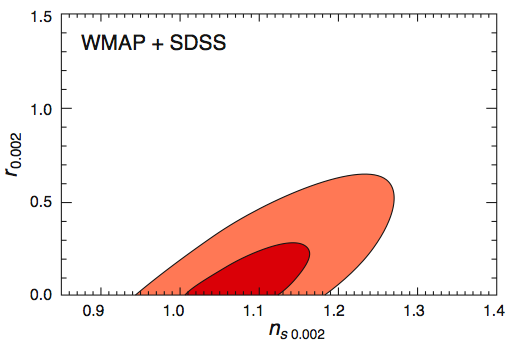
and choosing the upper right-hand corner of the 1-σ ellipse from the WMAP3+SDSS data, one finds ${𝒩}_{\text{eff}}\gtrsim 30$, which turns (4) into a lower bound on the excursion of the inflaton in field space. $$\frac{r_{\text{CMB}}}{0.01}\lesssim \frac{8}{9}{\left(\frac{\Delta \varphi }{M_p}\right)}^2$$

The clear implication is that, if they see a signal, it implies Planckian excursion in field space.

As Baumann and McAllister found, this proves to be surprisingly hard to achieve in string theory.

The most popular mechanism for inflation in string theory is D-brane inflation. The inflaton is the position of a D3-brane, as it moves down a warped throat. One might think that one can arrange for a very long, “narrow” throat, and thereby a large excursion in field space.

In a warped flux compactification of Type IIB down to 4 dimensions, the 10D metric takes the form $${ds}^2=h(y{)}^{-1/2}{g}_{\mu \nu }(x)d{x}^{\mu }d{x}^{\nu }+h(y{)}^{1/2}{g}_{ij}(y)d{y}^{i}d{y}^j$$ We are interested in the throat region, where the metric on the Calabi-Yau takes the form of a cone $$g_{ij}(y)d{y}^{i}d{y}^j=d{\rho }^2+{\rho }^2{ds}_{X_5}^2$$ over a Sasaki-Einstein 5-manifold, $X_5$. At least for some range of $\rho$, the geometry is that of AdS₅$\times X_5$, $$h(\rho )={\left(\frac{R}{\rho }\right)}^4$$ where $$R^4=4\pi g_s{(\alpha \prime )}^{2}N\frac{{\pi }^3}{\mathrm{Vol}(X_5)}$$ and $N$ is the dissolved D3-brane charge (the $F_5$ flux on $X_5$).

We should cut this off near the tip of the cone ($\rho >{\rho }_{\text{IR}}$), where the supergravity approximation breaks down, and at $\rho <{\rho }_{\text{UV}}$, where the geometry merges into that of the bulk Calabi-Yau.

The 4D Planck mass,

where $$V_6^w=\int d^{6}y\sqrt{g(y)}h(y)$$ A lower bound on $M_p^2>\frac{(V_6^w{)}_{\text{throat}}}{{\kappa }_{10}^2}$ can be obtained by just integrating over the throat region

Note that $\mathrm{Vol}(X_5)$ has dropped out, and the result depends only on $N$.

The canonically-normalized inflaton field is

Combining (6), (7), (8) and ${(\Delta \varphi )}^2<T_3{\rho }_{\text{UV}}^2$, we obtain the remarkably simple result

Since obtaining a warped throat region, in the first place, requires $N\gg 1$, we see that, quite robustly, the inflaton can’t have Planckian excursions in field space.

Of course, slow-roll is not the only possibility for D-brane inflation. Another possibility is DBI inflation. They consider a general class of models, $$S=\frac{1}{2}\int d^{4}x\sqrt{-g}(M_p^{2}R+2P(Y,\varphi )),Y=-\frac{1}{2}{g}^{\mu \nu }{\partial }_{\mu }\varphi {\partial }_{\nu }\varphi$$ that interpolate between the two. For all of these models, the derivation of the Lyth bound (4) goes through unaltered. The only modification comes in the evolution of $r(𝒩)$, where (5) is replaced by $$\frac{d\log r}{d𝒩}=n_t-(n_s-1)=-[(n_s-1)+\frac{r}{8c_s}]$$ where $c_s$ is the speed of sound of the model, $$c_s^2=\frac{dP}{d\rho }=\frac{\partial P/\partial Y}{\partial \rho /\partial Y}$$ and $\rho =2Y\partial P/\partial Y-P$ is the energy density.

Other models of inflation in string theory, involving, say, some closed-string modulus as the inflaton, seem to lead to the same conclusion.

The only model which might conceivably give a detectable tensor signal is N-flation, or, as it might better be called, “axion assisted inflation,” in which one has a large number of scalar fields (natural candidates are the axions which are the superpartners of the Kähler moduli in the aformentioned Type-IIB flux compactifications.) roll simultaneously.

The idea of assisted inflation is that, if you have a large number, $N$, of scalar field, whose potentials are, individually, too steep to support slow-roll inflation, they may, nonetheless undergo slow-roll if they all roll simultaneously, since the Hubble friction is common to them, and $H\sim N^{1/2}$.

Easther and McAllister have an elegant twist on this, in which the potential for these axions is given by a random matrix model. If the entries obey the Marčenko-Pastur distribution (which seems to arise naturally from the form of the supergravity action), then one may be able to generate an observable $r$.

But, I’m afraid I’ll have to postpone discussion of that to another post …

---