Dear Twitter Anti-Zionists,
For five months, ever since Oct. 7, I’ve read you obsessively. While my current job is supposed to involve protecting humanity from the dangers of AI (with a side of quantum computing theory), I’m ashamed to say that half the days I don’t do any science; instead I just scroll and scroll, reading anti-Israel content and then pro-Israel content and then more anti-Israel content. I thought refusing to post on Twitter would save me from wasting my life there as so many others have, but apparently it doesn’t, not anymore. (No, I won’t call it “X.”)
At the high end of the spectrum, I religiously check the tweets of Paul Graham, a personal hero and inspiration to me ever since he wrote Why Nerds Are Unpopular twenty years ago, and a man with whom I seem to resonate deeply on every important topic except for two: Zionism and functional programming. At the low end, I’ve read hundreds of the seemingly infinite army of Tweeters who post images of hook-nosed rats with black hats and sidecurls and dollar signs in their eyes, sneering as they strangle the earth and stab Palestinian babies. I study their detailed theories about why the October 7 pogrom never happened, and also it was secretly masterminded by Israel just to create an excuse to mass-murder Palestinians, and also it was justified and thrilling (exactly the same melange long ago embraced for the Holocaust).
I’m aware, of course, that the bottom-feeders make life too easy for me, and that a single Paul Graham who endorses the anti-Zionist cause ought to bother me more than a billion sharers of hook-nosed rat memes. And he does. That’s why, in this letter, I’ll try to stay at the higher levels of Graham’s Disagreement Hierarchy.
More to the point, though, why have I spent so much time on such a depressing, unproductive reading project?
Damned if I know. But it’s less surprising when you recall that, outside theoretical computer science, I’m (alas) mostly known to the world for having once confessed, in a discussion deep in the comment section of this blog, that I spent much of my youth obsessively studying radical feminist literature. I explained that I did that because my wish, for a decade, was to confront progressivism’s highest moral authorities on sex and relationships, and make them tell me either that
(1) I, personally, deserved to die celibate and unloved, as a gross white male semi-autistic STEM nerd and stunted emotional and aesthetic cripple, or else
(2) no, I was a decent human being who didn’t deserve that.
One way or the other, I sought a truthful answer, one that emerged organically from the reigning morality of our time and that wasn’t just an unprincipled exception to it. And I felt ready to pursue progressive journalists and activists and bloggers and humanities professors to the ends of the earth before I’d let them leave this one question hanging menacingly over everything they’d ever written, with (I thought) my only shot at happiness in life hinging on their answer to it.
You might call this my central character flaw: this need for clarity from others about the moral foundations of my own existence. I’m self-aware enough to know that it is a severe flaw, but alas, that doesn’t mean that I ever figured out how to fix it.
It’s been exactly the same way with the anti-Zionists since October 7. Every day I read them, searching for one thing and one thing only: their own answer to the “Jewish Question.” How would they ensure that the significant fraction of the world that yearns to murder all Jews doesn’t get its wish in the 21st century, as to a staggering extent it did in the 20th? I confess to caring about that question, partly (of course) because of the accident of having been born a Jew, and having an Israeli wife and family in Israel and so forth, but also because, even if I’d happened to be a Gentile, the continued survival of the world’s Jews would still seem remarkably bound up with science, Enlightenment, minority rights, liberal democracy, meritocracy, and everything else I’ve ever cared about.
I understand the charges against me. Namely: that if I don’t call for Israel to lay down its arms right now in its war against Hamas (and ideally: to dissolve itself entirely), then I’m a genocidal monster on the wrong side of history. That I value Jewish lives more than Palestinian lives. That I’m a hasbara apologist for the IDF’s mass-murder and apartheid and stealing of land. That if images of children in Gaza with their limbs blown off, or dead in their parents arms, or clawing for bread, don’t cause to admit that Israel is evil, then I’m just as evil as the Israelis are.
Unsurprisingly I contest the charges. As a father of two, I can no longer see any images of child suffering without thinking about my own kids. For all my supposed psychological abnormality, the part of me that’s horrified by such images seems to be in working order. If you want to change my mind, rather than showing me more such images, you’ll need to target the cognitive part of me: the part that asks why so many children are suffering, and what causal levers we’d need to push to reach a place where neither side’s children ever have to suffer like this ever again.
At risk of stating the obvious: my first-order model is that Hamas, with the diabolical brilliance of a Marvel villain, successfully contrived a situation where Israel could prevent the further massacring of its own population only by fighting a gruesome urban war, of a kind that always, anywhere in the world, kills tens of thousands of civilians. Hamas, of course, was helped in this plan by an ideology that considers martyrdom the highest possible calling for the innocents who it rules ruthlessly and hides underneath. But Hamas also understood that the images of civilian carnage would (rightly!) shock the consciences of Israel’s Western allies and many Israelis themselves, thereby forcing a ceasefire before the war was over, thereby giving Hamas the opportunity to regroup and, with God’s and of course Iran’s help, finally finish the job of killing all Jews another day.
And this is key: once you remember why Hamas launched this war and what its long-term goals are, every detail of Twitter’s case against Israel has to be reexamined in a new light. Take starvation, for example. Clearly the only explanation for why Israelis would let Gazan children starve is the malice in their hearts? Well, until you think through the logistical challenges of feeding 2.3 million starving people whose sole governing authority is interested only in painting the streets red with Jewish blood. Should we let that authority commandeer the flour and water for its fighters, while innocents continue to starve? No? Then how about UNRWA? Alas, we learned that UNRWA, packed with employees who cheered the Oct. 7 massacre in their Telegram channels and in some cases took part in the murders themselves, capitulates to Hamas so quickly that it effectively is Hamas. So then Israel should distribute the food itself! But as we’ve dramatically witnessed, Israel can’t distribute food without imposing order, which would seem to mean reoccupying Gaza and earning the world’s condemnation for it. Do you start to appreciate the difficulty of the problem—and why the Biden administration was pushed to absurd-sounding extremes like air-dropping food and then building a floating port?
It all seems so much easier, once you remove the constraint of not empowering Hamas in its openly-announced goal of completing the Holocaust. And hence, removing that constraint is precisely what the global left does.
For all that, by Israeli standards I’m firmly in the anti-Netanyahu, left-wing peace camp—exactly where I’ve been since the 1990s, as a teenager mourning the murder of Rabin. And I hope even the anti-Israel side might agree with me that, if all the suffering since Oct. 7 has created a tiny opening for peace, then walking through that opening depends on two things happening:
- the removal of Netanyahu, and
- the removal of Hamas.
The good news is that Netanyahu, the catastrophically failed “Protector of Israel,” not only can, but plausibly will (if enough government ministers show some backbone), soon be removed in a democratic election.
Hamas, by contrast, hasn’t allowed a single election since it took power in 2006, in a process notable for its opponents being thrown from the roofs of tall buildings. That’s why even my left-leaning Israeli colleagues—the ones who despise Netanyahu, who marched against him last year—support Israel’s current war. They support it because, even if the Israeli PM were Fred Rogers, how can you ever get to peace without removing Hamas, and how can you remove Hamas except by war, any more than you could cut a deal with Nazi Germany?
I want to see the IDF do more to protect Gazan civilians—despite my bitter awareness of survey data suggesting that many of those civilians would murder my children in front of me if they ever got a chance. Maybe I’d be the same way if I’d been marinated since birth in an ideology of Jew-killing, and blocked from other sources of information. I’m heartened by the fact that despite this, indeed despite the risk to their lives for speaking out, a full 15% of Gazans openly disapprove of the Oct. 7 massacre. I want a solution where that 15% becomes 95% with the passing of generations. My endgame is peaceful coexistence.
But to the anti-Zionists I say: I don’t even mind you calling me a baby-eating monster, provided you honestly field one question. Namely:
Suppose the Palestinian side got everything you wanted for it; then what would be your plan for the survival of Israel’s Jews?
Let’s assume that not only has Netanyahu lost the next election in a landslide, but is justly spending the rest of his life in Israeli prison. Waving my wand, I’ve made you Prime Minister in his stead, with an overwhelming majority in the Knesset. You now get to go down in history as the liberator of Palestine. But you’re now also in charge of protecting Israel’s 7 million Jews (and 2 million other residents) from near-immediate slaughter at the hands of those who you’ve liberated.
Granted, it seems pretty paranoid to expect such a slaughter! Or rather: it would seem paranoid, if the Palestinians’ Grand Mufti (progenitor of the Muslim Brotherhood and hence Hamas) hadn’t allied himself with Hitler in WWII, enthusiastically supported the Nazi Final Solution, and tried to export it to Palestine; if in 1947 the Palestinians hadn’t rejected the UN’s two-state solution (the one Israel agreed to) and instead launched another war to exterminate the Jews (a war they lost); if they hadn’t joined the quest to exterminate the Jews a third time in 1967; etc., or if all this hadn’t happened back before there were any settlements or occupation, when the only question on the table was Israel’s existence. It would seem paranoid if Arafat had chosen a two-state solution when Israel offered it to him at Camp David, rather than suicide bombings. It would seem paranoid if not for the candies passed out in the streets in celebration on October 7.
But if someone has a whole ideology, which they teach their children and from which they’ve never really wavered for a century, about how murdering you is a religious honor, and also they’ve actually tried to murder you at every opportunity—-what more do you want them to do, before you’ll believe them?
So, you tell me your plan for how to protect Israel’s 7 million Jews from extermination at the hands of neighbors who have their extermination—my family’s extermination—as their central political goal, and who had that as their goal long before there was any occupation of the West Bank or Gaza. Tell me how to do it while protecting Palestinian innocents. And tell me your fallback plan if your first plan turns out not to work.
We can go through the main options.
(1) UNILATERAL TWO-STATE SOLUTION
Maybe your plan is that Israel should unilaterally dismantle West Bank settlements, recognize a Palestinian state, and retreat to the 1967 borders.
This is an honorable plan. It was my preferred plan—until the horror of October 7, and then the even greater horror of the worldwide left reacting to that horror by sharing celebratory images of paragliders, and by tearing down posters of kidnapped Jewish children.
Today, you might say October 7 has sort of put a giant flaming-red exclamation point on what’s always been the central risk of unilateral withdrawal. Namely: what happens if, afterward, rather than building a peaceful state on their side of the border, the Palestinian leadership chooses instead to launch a new Iran-backed war on Israel—one that, given the West Bank’s proximity to Israel’s main population centers, makes October 7 look like a pillow fight?
If that happens, will you admit that the hated Zionists were right and you were wrong all along, that this was never about settlements but always, only about Israel’s existence? Will you then agree that Israel has a moral prerogative to invade the West Bank, to occupy and pacify it as the Allies did Germany and Japan after World War II? Can I get this in writing from you, right now? Or, following the future (October 7)2 launched from a Judenfrei West Bank, will your creativity once again set to work constructing a reason to blame Israel for its own invasion—because you never actually wanted a two-state solution at all, but only Israel’s dismantlement?
(2) NEGOTIATED TWO-STATE SOLUTION
So, what about a two-state solution negotiated between the parties? Israel would uproot all West Bank settlements that prevent a Palestinian state, and resettle half a million Jews in pre-1967 Israel—in exchange for the Palestinians renouncing their goal of ending Israel’s existence, via a “right of return” or any other euphemism.
If so: congratulations, your “anti-Zionism” now seems barely distinguishable from my “Zionism”! If they made me the Prime Minister of Israel, and put you in charge of the Palestinians, I feel optimistic that you and I could reach a deal in an hour and then go out for hummus and babaganoush.
(3) SECULAR BINATIONAL STATE
In my experience, in the rare cases they deign to address the question directly, most anti-Zionists advocate a “secular, binational state” between the Jordan and Mediterranean, with equal rights for all inhabitants. Certainly, that would make sense if you believe that Israel is an apartheid state just like South Africa.
To me, though, this analogy falls apart on a single question: who’s the Palestinian Nelson Mandela? Who’s the Palestinian leader who’s ever said to the Jews, “end your Jewish state so that we can live together in peace,” rather than “end your Jewish state so that we can end your existence”? To impose a binational state would be to impose something, not only that Israelis regard as an existential horror, but that most Palestinians have never wanted either.
But, suppose we do it anyway. We place 7 million Jews, almost half the Jews who remain on Earth, into a binational state where perhaps a third of their fellow citizens hold the theological belief that all Jews should be exterminated, and that a heavenly reward follows martyrdom in blowing up Jews. The exterminationists don’t quite have a majority, but they’re the second-largest voting bloc. Do you predict that the exterminationists will give up their genocidal ambition because of new political circumstances that finally put their ambition within reach? If October-7 style pogroms against Jews turn out to be a regular occurrence in our secular binational state, how will its government respond—like the Palestinian Authority? like UNRWA? like the British Mandate? like Tsarist Russia?
In such a case, perhaps the Jews (along with those Arabs and Bedouins and Druze and others who cast their lot with the Jews) would need form a country-within-a-country: their own little autonomous zone within the binational state, with its own defense force. But of course, such a country-within-a-country already formed, for pretty much this exact reason. It’s called Israel. A cycle has been detected in your arc of progress.
(4) EVACUATION OF THE JEWS FROM ISRAEL
We come now to the anti-Zionists who are plainspoken enough to say: Israel’s creation was a grave mistake, and that mistake must now be reversed.
This is a natural option for anyone who sees Israel as an “illegitimate settler-colonial project,” like British India or French Algeria, but who isn’t quite ready to call for another Jewish genocide.
Again, the analogy runs into obvious problems: Israelis would seem to be the first “settler-colonialists” in the history of the world who not only were indigenous to the land they colonized, as much as anyone was, but who weren’t colonizing on behalf of any mother country, and who have no obvious such country to which they can return.
Some say spitefully: then let the Jews go back to Poland. These people might be unaware that, precisely because of how thorough the Holocaust was, more Israeli Jews trace their ancestry to Muslim countries than to Europe. Is there to be a “right of return” to Egypt, Iraq, Morocco, and Yemen, for all the Jews forcibly expelled from those places and for their children and grandchildren?
Others, however, talk about evacuating the Jews from Israel with goodness in their hearts. They say: we’d love the Israelis’ economic dynamism here in Austin or Sydney or Oxfordshire, joining their many coreligionists who already call these places home. What’s more, they’ll be safer here—who wants to live with missiles raining down on their neighborhood? Maybe we could even set aside some acres in Montana for a new Jewish homeland.
Again, if this is your survival plan, I’m a billion times happier to discuss it openly than to have it as unstated subtext!
Except, maybe you could say a little more about the logistics. Who will finance the move? How confident are you that the target country will accept millions of defeated, desperate Jews, as no country on earth was the last time this question arose?
I realize it’s no longer the 1930s, and Israel now has friends, most famously in America. But—what’s a good analogy here? I’ve met various Silicon Valley gazillionaires. I expect that I could raise millions from them, right now, if I got them excited about a new project in quantum computing or AI or whatever. But I doubt I could raise a penny from them if I came to them begging for their pity or their charity.
Likewise: for all the anti-Zionists’ loudness, a solid majority of Americans continue to support Israel (which, incidentally, provides a much simpler explanation than the hook-nosed perfidy of AIPAC for why Congress and the President mostly support it). But it seems to me that Americans support Israel in the “exciting project” sense, rather than in the “charity” sense. They like that Israelis are plucky underdogs who made the deserts bloom, and built a thriving tech industry, and now produce hit shows like Shtisel and Fauda, and take the fight against a common foe to the latter’s doorstep, and maintain one of the birthplaces of Western civilization for tourists and Christian pilgrims, and restarted the riveting drama of the Bible after a 2000-year hiatus, which some believe is a crucial prerequisite to the Second Coming.
What’s important, for present purposes, is not whether you agree with any of these rationales, but simply that none of them translate into a reason to accept millions of Jewish refugees.
But if you think dismantling Israel and relocating its seven million Jews is a workable plan—OK then, are you doing anything to make that more than a thought experiment, as the Zionists did a century ago with their survival plan? Have even I done more to implement your plan than you have, by causing one Israeli (my wife) to move to the US?
Suppose you say it’s not your job to give me a survival plan for Israel’s Jews. Suppose you say the request is offensive, an attempt to distract from the suffering of the Palestinians, so you change the subject.
In that case, fine, but you can now take off your cloak of righteousness, your pretense of standing above me and judging me from the end of history. Your refusal to answer the question amounts to a confession that, for you, the goal of “a free Palestine from the river to the sea” doesn’t actually require the physical survival of Israel’s Jews.
Which means, we’ve now established what you are. I won’t give you the satisfaction of calling you a Nazi or an antisemite. Thousands of years before those concepts existed, Jews already had terms for you. The terms tended toward a liturgical register, as in “those who rise up in every generation to destroy us.” The whole point of all the best-known Jewish holidays, like Purim yesterday, is to talk about those wicked would-be destroyers in the past tense, with the very presence of live Jews attesting to what the outcome was.
(Yesterday, I took my kids to a Purim carnival in Austin. Unlike in previous years, there were armed police everywhere. It felt almost like … visiting Israel.)
If you won’t answer the question, then it wasn’t Zionist Jews who told you that their choices are either to (1) oppose you or else (2) go up in black smoke like their grandparents did. You just told them that yourself.
Many will ask: why don’t I likewise have an obligation to give you my Palestinian survival plan?
I do. But the nice thing about my position is that I can tell you my Palestinian survival plan cheerfully, immediately, with zero equivocating or changing the subject. It’s broadly the same plan that David Ben-Gurion and Yitzchak Rabin and Ehud Barak and Bill Clinton and the UN put on the table over and over and over, only for the Palestinians’ leaders to sweep it off.
I want the Palestinians to have a state, comprising the West Bank and Gaza, with a capital in East Jerusalem. I want Israel to uproot all West Bank settlements that prevent such a state. I want this to happen the instant there arises a Palestinian leadership genuinely committed to peace—one that embraces liberal values and rejects martyr values, in everything from textbooks to street names.
And I want more. I want the new Palestinian state to be as prosperous and free and educated as modern Germany and Japan are. I want it to embrace women’s rights and LGBTQ+ rights and the rest of the modern package, so that “Queers for Palestine” would no longer be a sick joke. I want the new Palestine to be as intertwined with Israel, culturally and economically, as the US and Canada are.
Ironically, if this ever became a reality, then Israel-as-a-Jewish-state would no longer be needed—but it’s certainly needed in the meantime.
Anti-Zionists on Twitter: can you be equally explicit about what you want?
I come, finally, to what many anti-Zionists regard as their ultimate trump card. Look at all the anti-Zionist Jews and Israelis who agree with us, they say. Jewish Voice for Peace. IfNotNow. Noam Chomsky. Norman Finkelstein. The Neturei Karta.
Intellectually, of course, the fact of anti-Zionist Jews makes not the slightest difference to anything. My question for them remains exactly the same as for anti-Zionist Gentiles: what is your Jewish survival plan, for the day after we dismantle the racist supremacist apartheid state that’s currently the only thing standing between half the world’s remaining Jews and their slaughter by their neighbors? Feel free to choose from any of the four options above, or suggest a fifth.
But in the event that Jewish anti-Zionists evade that conversation, or change the subject from it, maybe some special words are in order. You know the famous Golda Meir line, “If we have to choose between being dead and pitied and being alive with a bad image, we’d rather be alive and have the bad image”?
It seems to me that many anti-Zionist Jews considered Golda Meir’s question carefully and honestly, and simply decided it the other way, in favor of Jews being dead and pitied.
Bear with me here: I won’t treat this as a reductio ad absurdum of their position. Not even if the anti-Zionist Jews themselves wish to remain safely ensconced in Berkeley or New Haven, while the Israelis fulfill the “dead and pitied” part for them.
In fact, I’ll go further. Again and again in life I’ve been seized by a dark thought: if half the world’s Jews can only be kept alive, today, via a militarized ethnostate that constantly needs to defend its existence with machine guns and missiles, racking up civilian deaths and destabilizing the world’s geopolitics—if, to put a fine point on it, there are 16 million Jews in the world, but at least a half billion antisemites who wake up every morning and go to sleep every night desperately wishing those Jews dead—then, from a crude utilitarian standpoint, might it not be better for the world if we Jews vanished after all?
Remember, I’m someone who spent a decade asking myself whether the rapacious, predatory nature of men’s sexual desire for women, which I experienced as a curse and an affliction, meant that the only moral course for me was to spend my life as a celibate mathematical monk. But I kept stumbling over one point: why should such a moral obligation fall on me alone? Why doesn’t it fall on other straight men, particularly the ones who presume to lecture me on my failings?
And also: supposing I did take the celibate monk route, would even that satisfy my haters? Would they come after me anyway for glancing at a woman too long or making an inappropriate joke? And also: would the haters soon say I shouldn’t have my scientific career either, since I’ve stolen my coveted academic position from the underprivileged? Where exactly does my self-sacrifice end?
When I did, finally, start approaching women and asking them out on dates, I worked up the courage partly by telling myself: I am now going to do the Zionist thing. I said: if other nerdy Jews can risk death in war, then this nerdy Jew can risk ridicule and contemptuous stares. You can accept that half the world will denounce you as a monster for living your life, so long as your own conscience (and, hopefully, the people you respect the most) continue to assure you that you’re nothing of the kind.
This took more than a decade of internal struggle, but it’s where I ended up. And today, if anyone tells me I had no business ever forming any romantic attachments, I have two beautiful children as my reply. I can say: forget about me, you’re asking for my children never to have existed—that’s why I’m confident you’re wrong.
Likewise with the anti-Zionists. When the Twitter-warriors share their memes of hook-nosed Jews strangling the planet, innocent Palestinian blood dripping from their knives, when the global protests shut down schools and universities and bridges and parliament buildings, there’s a part of me that feels eager to commit suicide if only it would appease the mob, if only it would expiate all the cosmic guilt they’ve loaded onto my shoulders.
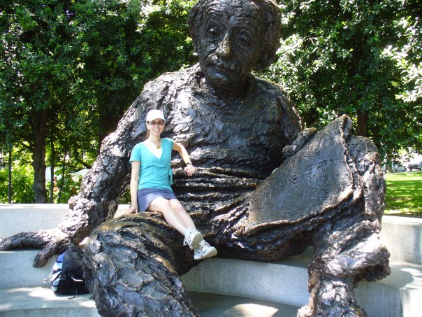
But then I remember that this isn’t just about me. It’s about Einstein and Spinoza and Feynman and Erdös and von Neumann and Weinberg and Landau and Michelson and Rabi and Tarski and Asimov and Sagan and Salk and Noether and Meitner, and Irving Berlin and Stan Lee and Rodney Dangerfield and Steven Spielberg. Even if I didn’t happen to be born Jewish—if I had anything like my current values, I’d still think that so much of what’s worth preserving in human civilization, so much of math and science and Enlightenment and democracy and humor, would seem oddly bound up with the continued survival of this tiny people. And conversely, I’d think that so much of what’s hateful in civilization would seem oddly bound up with the quest to exterminate this tiny people, or to deny it any means to defend itself from extermination.
So that’s my answer, both to anti-Zionist Gentiles and to anti-Zionist Jews. The problem of Jewish survival, on a planet much of which yearns for the Jews’ annihilation and much of the rest of which is indifferent, is both hard and important, like P versus NP. And so a radical solution was called for. The solution arrived at a century ago, at once brand-new and older than Homer and Hesiod, was called the State of Israel. If you can’t stomach that solution—if, in particular, you can’t stomach the violence needed to preserve it, so long as Israel’s neighbors retain their annihilationist dream—then your response ought to be to propose a better solution. I promise to consider your solution in good faith—asking, just like with P vs. NP provers, how you overcome the problems that doomed all previous attempts. But if you throw my demand for a better solution back in my face, then you might as well be pushing my kids into a gas chamber yourself, for all the moral authority that I now recognize you to have over me.
Possibly the last thing Einstein wrote was a speech celebrating Israel’s 7th Independence Day, which he died a week before he was to deliver. So let’s turn the floor over to Mr. Albert, the leftist pacifist internationalist:
This is the seventh anniversary of the establishment of the State of Israel. The establishment of this State was internationally approved and recognised largely for the purpose of rescuing the remnant of the Jewish people from unspeakable horrors of persecution and oppression.
Thus, the establishment of Israel is an event which actively engages the conscience of this generation. It is, therefore, a bitter paradox to find that a State which was destined to be a shelter for a martyred people is itself threatened by grave dangers to its own security. The universal conscience cannot be indifferent to such peril.
It is anomalous that world opinion should only criticize Israel’s response to hostility and should not actively seek to bring an end to the Arab hostility which is the root cause of the tension.
I love Einstein’s use of “anomalous,” as if this were a physics problem. From the standpoint of history, what’s anomalous about the Israeli-Palestinian conflict is not, as the Twitterers claim, the brutality of the Israelis—if you think that’s anomalous, you really haven’t studied history—but something different. In other times and places, an entity like Palestine, which launches a war of total annihilation against a much stronger neighbor, and then another and another, would soon disappear from the annals of history. Israel, however, is held to a different standard. Again and again, bowing to international pressure and pressure from its own left flank, the Israelis have let their would-be exterminators off the hook, bruised but mostly still alive and completely unrepentant, to have another go at finishing the Holocaust in a few years. And after every bout, sadly but understandably, Israeli culture drifts more to the right, becomes 10% more like the other side always was.
I don’t want Israel to drift to the right. I find the values of Theodor Herzl and David Ben-Gurion to be almost as good as any human values have ever been, and I’d like Israel to keep them. Of course, Israel will need to continue defending itself from genocidal neighbors, until the day that a leader arises among the Palestinians with the moral courage of Egypt’s Anwar Sadat or Jordan’s King Hussein: a leader who not only talks peace but means it. Then there can be peace, and an end of settlements in the West Bank, and an independent Palestinian state. And however much like dark comedy that seems right now, I’m actually optimistic that it will someday happen, conceivably even soon depending on what happens in the current war. Unless nuclear war or climate change or AI apocalypse makes the whole question moot.
Anyway, thanks for reading—a lot built up these past months that I needed to get off my chest. When I told a friend that I was working on this post, he replied “I agree with you about Israel, of course, but I choose not to die on that hill in public.” I answered that I’ve already died on that hill and on several other hills, yet am somehow still alive!
Meanwhile, I was gratified that other friends, even ones who strongly disagree with me about Israel, told me that I should not disengage, but continue to tell it like I see it, trying civilly to change minds while being open to having my own mind changed.
And now, maybe, I can at last go back to happier topics, like how to prevent the destruction of the world by AI.
Cheers,
Scott
.")

 , and a subset
  of
of  , we define the
 of
of  in
in  to be the set of all pairs
  where
where  are distinct elements of
 ![{[G:2G]}](https://s0.wp.com/latex.php?latex=%7B%5BG%3A2G%5D%7D&bg=ffffff&fg=000000&s=0&c=20201002) finite. Let
finite. Let  and
and  such that
  .
.  , but as noted in the recent preprint of
  has finite index. This condition is in fact necessary (as observed by forthcoming work of Ethan Acklesberg): if
  has infinite index, then one can find a subgroup
  of
of  for any
  that contains
  is
is  -torsion). If one lets
  be an enumeration of
 for any
  (indeed, from the pigeonhole principle and the
  one can show that
  must intersect
  whenever
  ). It is also necessary to work with restricted sums
  : a counterexample to the latter is provided for instance by the example with
  and
and ![{A := \bigcup_{j=1}^\infty [10^j, 1.1 \times 10^j]}](https://s0.wp.com/latex.php?latex=%7BA+%3A%3D+%5Cbigcup_%7Bj%3D1%7D%5E%5Cinfty+%5B10%5Ej%2C+1.1+%5Ctimes+10%5Ej%5D%7D&bg=ffffff&fg=000000&s=0&c=20201002) . Finally, the presence of the shift
. Finally, the presence of the shift  , though in the case
  one can of course delete the shift
  is a compact topological space (with the topology of pointwise convergence) (it is also metrizable since
  of
of  can be thought of as properties of subsets of
  that shares a sufficiently large (but finite) initial segment with
  elements.
  elements, where
  elements, where
  is the
  element of
  halts when given
  an
an  be a Følner sequence in
  , and let
  be a largeness property for each integer
  such that if
  is such that
  for all
  , then there exists a shift
  ,
,  ,
,  with
with  for all
  . By compactness, a subsequence of the
  . By openness, we conclude that there exists a finite
  . This implies that
  for infinitely many
  be as in Theorem
  between
  by declaring
  if
if  is an open subset of
 , then
  , and then any
  that contains both
  lies in
  .
.  of subsets of
  in
in  converges pointwise to
  and
and  converges pointwise to
  . (By
. (By  of
of  for all sufficiently large
  and
and  be as in Theorem
  . Setting
  , we conclude that
  and
and  . Setting
  to be an even larger element of this sequence, we then have
  and
and  . Setting
  to be an even larger element, we have
  and
and  . Continuing in this fashion we obtain the desired infinite set
  to be a compact space
  equipped with a Borel probability measure
  as well as a measure-preserving homeomorphism
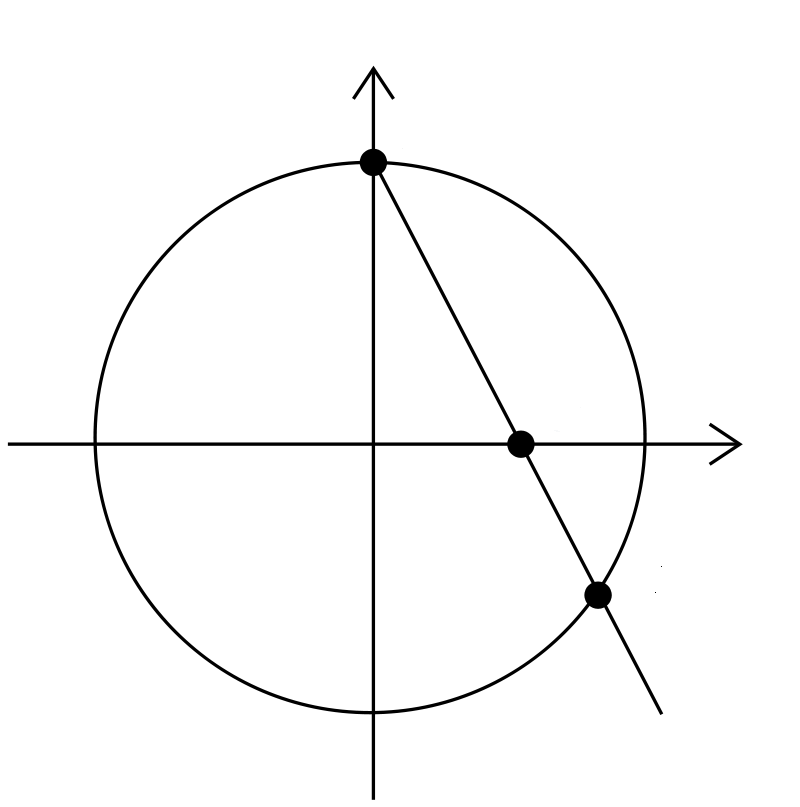
  . A point
  in
in  if one has
 . Define an (length three) dynamical Erdös progression to be a tuple
  in
in  and
and  .
.
 be a positive measure open subset of
  and
and  .
.  ,
,  , and
, and  for a Følner sequence
  with
with  , at which point Theorem
  of the Følner sequence are not required to contain the origin.)
 is a countable vector space over a finite field of size equal to an odd prime
  , so in particular
  ; we also specialize to Følner sequences of the form
  for some
  and
and  . In this case we can prove a stronger statement:
 for an odd prime
  be open subsets of
  . Then if
  , there exists an Erdös progression
  and
and  .
.  has full measure, so the hypothesis
  of Theorem
 ![{\mu(E_1)/[G:2G] + \mu(E_2) > 1}](https://s0.wp.com/latex.php?latex=%7B%5Cmu%28E_1%29%2F%5BG%3A2G%5D+%2B+%5Cmu%28E_2%29+%3E+1%7D&bg=ffffff&fg=000000&s=0&c=20201002) .)
.)
 be a compact metric space, let
  be a finite vector space over a field of odd prime order. Let
  , and let
  . Let
. Let  for some
  , there exist
  such that
 of open balls of radius
  . This induces a coloring function
  that assigns to each point in
  of the first ball
  that covers that point. This then induces a coloring
  of
of  . We also define the pullbacks
  for
for  . By hypothesis, we have
  , and it will now suffice by the triangle inequality to show that
 to be chosen later. This allows us to partition
  of index
  , such that on all but
 ![{\kappa [G:H]}](https://s0.wp.com/latex.php?latex=%7B%5Ckappa+%5BG%3AH%5D%7D&bg=ffffff&fg=000000&s=0&c=20201002) of these cosets
of these cosets  , all the color classes
  are
are  -regular in the Fourier (
 ) sense. Now we sample
  uniformly from
  ; as
; as  is also uniform in
  . By removing an exceptional event of probability
  , we may assume that neither of these cosetgs
  , we may also assume that
 . Similarly we may assume that


 -uniform in their respective cosets. Thus by standard Fourier calculations, we see that after excluding another exceptional event of probabitiy
 . By choosing
  small enough depending on
  , we can ensure that
  on
on  , we may assume that the
  grow as fast as we wish. Once we do so, we claim that for each
  , we can find
  such that for each
  , there exists
  that lies outside of
  such that
 converge to
  respectively, we obtain the desired Erdös progression.
 be a large parameter (much larger than
  converge vaguely to
  with
with  . Unfortunately,
  need not contain the origin.) However, we are assuming a continuous factor map
  to the Kronecker factor
  , which is a compact abelian group, and
  . As a consequence, we can find
  such that
  converges to
  converges to
  , so now
  converges vaguely to
  ,
,  , where
  is drawn uniformly at random from
  ,
,  ), but is easy to describe and will suffice for our argument. (A more appropriate choice, closer to the arguments of Kra et al., would be to
  , where the additional shift
  is a random variable in
  is a permutation on
  , and so

 denotes a quantity that goes to zero as
  (holding all other parameters fixed). By the hypothesis

 (compare with Theorem
  grow fast enough, we can then ensure that for each
  be the coloring function from the proof of Theorem
  ). Then it suffices to show that
 and
and  . This is a counting problem associated to the patterm
  ; if we concatenate the
  components of the pattern, this is a classic “complexity one” pattern, of the type that would be expected to be amenable to Fourier analysis (especially if one applies Cauchy-Schwarz to eliminate the
  ).
).
 of a level set of the coloring function
  is a bounded measurable function of
  that is measurable on the Kronecker factor, plus an error term
  that is orthogonal to that factor and thus is weakly mixing in the sense that
  tends to zero on average (or equivalently, that the Host-Kra seminorm
  vanishes). Meanwhile, for any
  , the Kronecker-measurable function
  , where
  is a bounded “trigonometric polynomial” (a finite sum of eigenfunctions) and
  . The polynomial
 , where
  is a bounded continuous function of
  norm at most
  , and
, and  is a bounded continuous function of
  (in practice we will take
  , we then have
 is just a sum of
  characters on
  such that these polynomial are constant on each coset of
  . Then
  and
and  . We then restrict
  to also lie in

 , which will establish our claim because
  .
.

 and
and  is annoying (as
  is an “infinite complexity” pattern that cannot be controlled by any uniformity norm), but (perhaps surprisingly) will not end up causing an essential difficulty to the argument, as we shall see when we start eliminating the terms in this sum one at a time starting from the right.
 term using
 , we may assume that the
  have normalized
  on both of these cosets
  . As such, the contribution of
  to
to  ). From the near weak mixing of the

 to
to  , if
, if  . Finally, the quantity
  is independent of
  in the coset
  . This density will be
  except for those
  which would have made a negligible impact on

 is small compared with
 of states,
 of transitions,
 mapping each transition to its upstream and downstream states.
 is the disjoint union of
  We get four cases:
 of agents. To handle births and deaths, I wanted to make this set time-dependent. But I need to separately say how this works for transformations, birth transitions and death transitions. For transformations we don’t change
  For birth transitions we add a new element to
  and maybe record its name on a ledger or drive a stake through its heart to make sure it can never be born again!
 agent
agent  arrives at the state upstream to some transition
  and the agents at states linked to the transition
  form some set
  when will agent
  , they don’t have a time at which they arrived at that state.
 in an unborn state. This can be done without using an infinite amount of memory: it’s a ‘potential infinity’ rather than an ‘actual infinity’.
 of vertices or states,
 of edges or transitions,
 mapping each edge to its source and target, also called its upstream and downstream,
 of links,
 and
and  mapping each link to its source (a state) and its target (a transition).
 will undergo a transition
  if it arrives at the state upstream to that transition at a specific time
  This jump function will not be deterministic: it will be a stochastic function, just as it was in
  and
and  But now the links will come into play.
 will have one state
  as its source. We say this state affects the transition
 So, we want the jump function for the transition
 And as mentioned earlier, the jump function will also depend on a choice of agent
 for each transition
 is the answer to this question:
 and the agents at states linked to the edge
  given that it doesn’t do anything else first?
 can keep changing. This is the big difference between today’s formalism and yesterday’s.
 namely:

 when will agent
 an agent makes a transition. More specifically, suppose agent
  makes a transition
  from the state


 (by removing
  from this subset) and in the state
  (by adding
  that’s affected by the state
 is the element of
  saying which subset of agents is in each state affecting the transition
  (So, we update our table of times at which agent
  given that it doesn’t do anything else first.)
 And we need to compute what actually happens then!
 for each agent
 replacing


 ︎
︎


 for all
  ), and let
  . Then
  translates of a subgroup
  . Moreover,
  for some
  .
. case of this result, with the number of translates bounded by
  (which was subsequently improved to
  by Jyun-Jie Liao), but without the additional containment
  . It remains a challenge to replace
  by a bounded constant (such as
  be independent finitely supported random variables on
 ![\displaystyle {\bf H}[X_1+\dots+X_m] - \frac{1}{m} \sum_{i=1}^m {\bf H}[X_i] \leq \log K,](https://s0.wp.com/latex.php?latex=%5Cdisplaystyle+%7B%5Cbf+H%7D%5BX_1%2B%5Cdots%2BX_m%5D+-+%5Cfrac%7B1%7D%7Bm%7D+%5Csum_%7Bi%3D1%7D%5Em+%7B%5Cbf+H%7D%5BX_i%5D+%5Cleq+%5Clog+K%2C&bg=ffffff&fg=000000&s=0&c=20201002)
 denotes Shannon entropy. Then there is a uniform random variable
  on a subgroup
 ![\displaystyle \frac{1}{m} \sum_{i=1}^m d[X_i; U_H] \ll m^3 \log K,](https://s0.wp.com/latex.php?latex=%5Cdisplaystyle+%5Cfrac%7B1%7D%7Bm%7D+%5Csum_%7Bi%3D1%7D%5Em+d%5BX_i%3B+U_H%5D+%5Cll+m%5E3+%5Clog+K%2C&bg=ffffff&fg=000000&s=0&c=20201002)
 take values in some symmetric set
  , then
  for some
  .
. of
of ![\displaystyle {\bf H}[X_1+\dots+X_m] - \frac{1}{m} \sum_{i=1}^m {\bf H}[X_i]](https://s0.wp.com/latex.php?latex=%5Cdisplaystyle+%7B%5Cbf+H%7D%5BX_1%2B%5Cdots%2BX_m%5D+-+%5Cfrac%7B1%7D%7Bm%7D+%5Csum_%7Bi%3D1%7D%5Em+%7B%5Cbf+H%7D%5BX_i%5D+&bg=ffffff&fg=000000&s=0&c=20201002)
 , but as we are not attempting to completely optimize the constants, we did not do so in the current paper (and as such, our arguments here give a slightly different way of establishing the
  random variables
  for
for  , with each
  of our array will end up being close to independent of the column sums
  , subject to conditioning on the total sum
  . Not coincidentally, this type of conditional independence phenomenon also shows up when considering row and column sums of iid independent gaussian random variables, as a specific feature of the gaussian distribution. It is related to the more familiar observation that if
  are two independent copies of a Gaussian random variable, then
  and
and  are also independent of each other.
 array of random variables as opposed to some other shape of array. But now the torsion enters in a key role, via the obvious identity
 ($1.048 million) has been allocated for various prizes associated to this competition. More detailed rules can be found


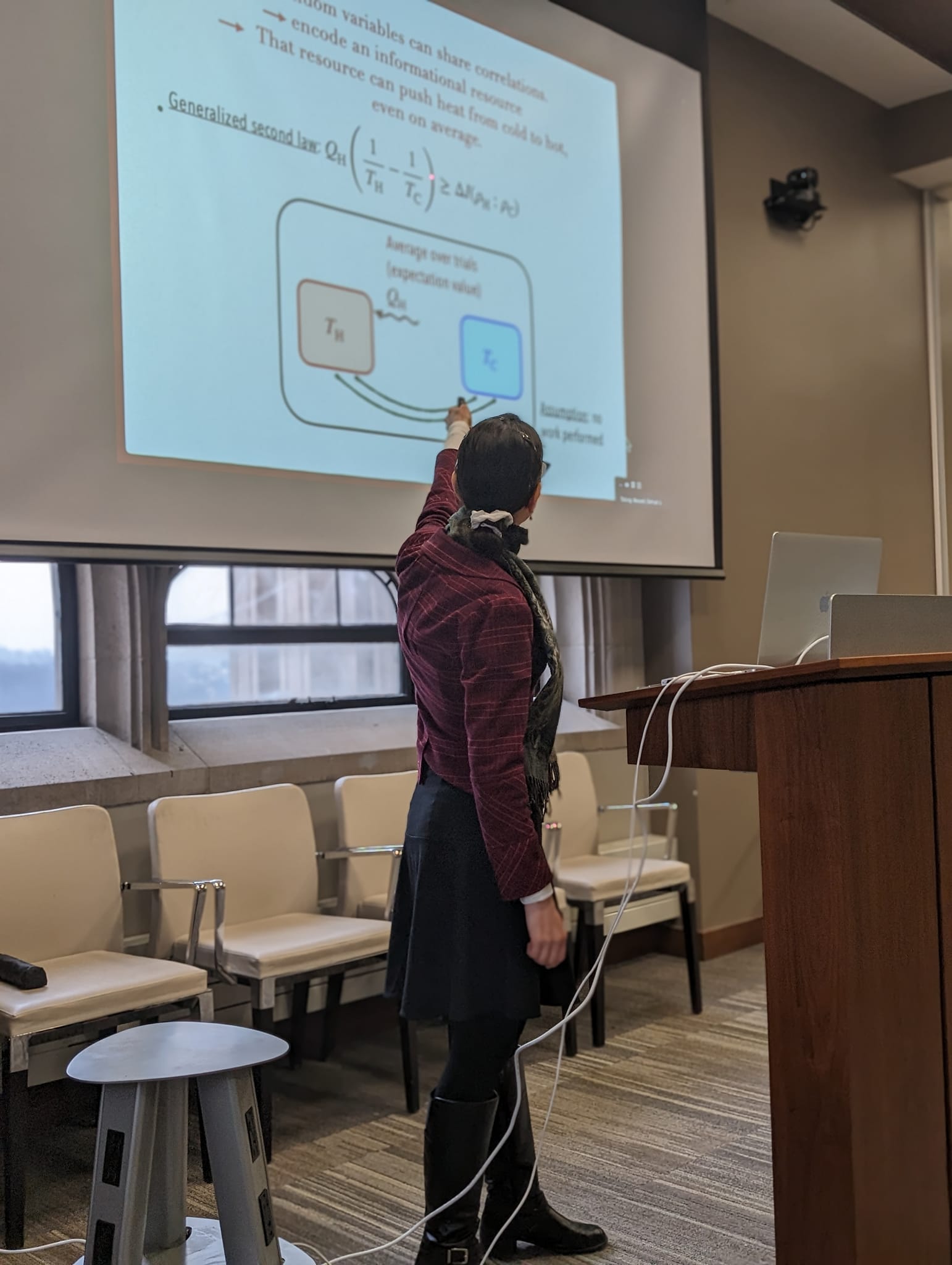
 . In Tucson, Arizona, even the airport has a saguaro crop sufficient for staging a Western short film. I didn’t have a film to shoot, but the garden set the stage for another adventure: the ITAMP winter school on quantum thermodynamics.


 .
.