The n-Category Café

Introduction

Bayesian networks are a graphical modelling tool used to show how random variables interact. A Bayesian network consists of a pair $(G,P)$ of directed acyclic graph (DAG) $G$ together with a joint probability distribution $P$ on its nodes, satisfying the Markov condition. Intuitively the graph describes a flow of information.

The Markov condition says that the system doesn’t have memory. That is, the distribution on a given node $Y$ is only dependent on the distributions on the nodes $X$ for which there is an edge $X \rightarrow Y$. Consider the following chain of binary events. In spring, the pollen in the air may cause someone to have an allergic reaction that may make them sneeze.

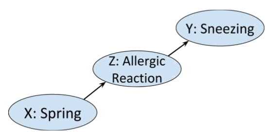
In this case the Markov condition says that given that you know that someone is having an allergic reaction, whether or not it is spring is not going to influence your belief about the likelihood of them sneezing. Which seems sensible.

Bayesian networks are useful

• as an inference tool, thanks to belief propagation algorithms,

• and because, given a Bayesian network $(G,P)$, we can describe ‘d-separation’ properties on $G$ which enable us to discover conditional independences in $P$.

It is this second point that we’ll be interested in here.

Before getting into the details of the paper, let’s try to motivate this discussion by explaining its title: “Theory-independent limits on correlations from generalized Bayesian networks" and giving a little more background to the problem it aims to solve.

Crudely put, the paper aims to generalise a method that assumes classical mechanics to one that holds in quantum and more general theories.

Classical mechanics rests on two intuitively reasonable and desirable assumptions, together called local causality,

• Causality:

  Causality is usually treated as a physical primitive. Simply put it is the principle that there is a (partial) ordering of events in space time. In order to have information flow from event $A$ to event $B$, $A$ must be in the past of $B$.

  Physicists often define causality in terms of a discarding principle: If we ignore the outcome of a physical process, it doesn’t matter what process has occurred. Or, put another way, the outcome of a physical process doesn’t change the initial conditions.

• Locality:

  Locality is the assumption that, at any given instant, the values of any particle’s properties are independent of any other particle. Intuitively, it says that particles are individual entities that can be understood in isolation of any other particle.

  Physicists usually picture particles as having a private list of numbers determining their properties. The principle of locality would be violated if any of the entries of such a list were a function whose domain is another particle’s property values.

In 1935 Einstein, Podolsky and Rosen showed that quantum mechanics (which was a recently born theory) predicted that a pair of particles could be prepared so that applying an action on one of them would instantaneously affect the other, no matter how distant in space they were, thus contradicting local causality. This seemed so unreasonable that the authors presented it as evidence that quantum mechanics was wrong.

But Einstein was wrong. In 1964, John S. Bell set the bases for an experimental test that would demonstrate that Einstein’s “spooky action at a distance” (Einstein’s own words), now known as entanglement, was indeed real. Bell’s experiment has been replicated countless of times and has plenty of variations. This video gives a detailed explanation of one of these experiments, for a non-physicist audience.

But then, if acting on a particle has an instantaneous effect on a distant point in space, one of the two principle above is violated: On one hand, if we acted on both particles at the same time, each action being a distinct event, both would be affecting each other’s result, so it would not be possible to decide on an ordering; causality would be broken. The other option would be to reject locality: a property’s value may be given by a function, so the resulting value may instantaneously change when the distant ‘domain’ particle is altered. In that case, the particles’ information was never separated in space, as they were never truly isolated, so causality is preserved.

Since causality is integral to our understanding of the world and forms the basis of scientific reasoning, the standard interpretation of quantum mechanics is to accept non-locality.

The definition of Bayesian networks implies a discarding principle and hence there is a formal sense in which they are causal (even if, as we shall see, the correlations they model do not always reflect the temporal order). Under this interpretation, the causal theory Bayesian networks describe is classical. Precisely, they can only model probability distributions that satisfy local causality. Hence, in particular, they are not sufficient to model all physical correlations.

The goal of the paper is to develop a framework that generalises Bayesian networks and d-separation results, so that we can still use graph properties to reason about conditional dependence under any given causal theory, be it classical, quantum, or even more general. In particular, this theory will be able to handle all physically observed correlations, and all theoretically postulated correlations.

Though category theory is not mentioned explicitly, the authors achieve their goal by using the categorical framework of operational probablistic theories (OPTs).

Bayesian networks and d-separation

Consider the situation in which we have three Boolean random variables. Alice is either sneezing or she is not, she either has a a fever or she does not, and she may or may not have flu.

Now, flu can cause both sneezing and fever, that is

$$P(sneezing \ | \ flu ) \neq P( sneezing) \ \text{ and likewise } \ P(fever \ | \ flu ) \neq P( fever)$$

so we could represent this graphically as

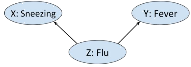
Moreover, intuitively we wouldn’t expect there to be any other edges in the above graph. Sneezing and fever, though correlated - each is more likely if Alice has flu - are not direct causes of each other. That is,

$$P(sneezing \ | \ fever ) \neq P(sneezing) \ \text{ but } \ P(sneezing \ | \ fever, \ flu ) = P(sneezing \ | \ flu).$$

Bayesian networks

Let $G$ be a directed acyclic graph or DAG $G$. (Here a directed graph is a presheaf on ($\bullet \rightrightarrows \bullet$)).

The set $Pa(Y)$ of parents of a node $Y$ of $G$ contains those nodes $X$ of $G$ such that there is a directed edge $X \to Y$.

So, in the example above $Pa(flu) = \emptyset$ while $Pa(fever) = Pa(sneezing) = \{ flu \}$.

To each node $X$ of a directed graph $G$, we may associate a random variable, also denoted $X$. If $V$ is the set of nodes of $G$ and $(x_X)_{X \in V}$ is a choice of value $x_X$ for each node $X$, such that $y$ is the chosen value for $Y$, then $pa(y)$ will denote the $Pa(Y)$-tuple of values $(x_X)_{X \in Pa(Y)}$.

To define Bayesian networks, and establish the notation, let’s revise some probability basics.

Let $P(x,y \ | \ z)$ mean $P(X = x \text{ and } \ Y = y \ | \ Z = z)$, the probability that $X$ has the value $x$, and $Y$ has the value $y$ given that $Z$ has the value $z$. Recall that this is given by

$$P(x,y \ |\ z) = \frac{ P(x,y,z) }{P(z)}.$$

The chain rule says that, given a value $x$ of $X$ and sets of values $\Omega, \Lambda$ of other random variables,

$$P(x, \Omega \ | \ \Lambda) = P( x \ | \ \Lambda) P( \Omega \ | \ x, \Lambda).$$

Random variables $X$ and $Y$ are said to be conditionally independent given $Z$, written $X \perp\!\!\!\!\!\!\!\perp Y \ | \ Z$, if for all values $x$ of $X$, $y$ of $Y$ and $z$ of $Z$

$$P(x,y \ | \ z) = P(x \ | \ z) P(y \ | \ z).$$

By the chain rule this is equivalent to

$$P(x \ | \ y,z ) = P (x \ | \ z) , \ \forall x,y, z.$$

More generally, we may replace $X,Y$ and $Z$ with sets of random variables. So, in the special case that $Z$ is empty, then $X$ and $Y$ are independent if and only if $P(x, y) = P(x)P(y)$ for all $x,y$.

Markov condition

A joint probability distribution $P$ on the nodes of a DAG $G$ is said to satisfy the Markov condition if for any set of random variable $\{X_i\}_{i = 1}^n$ on the nodes of $G$, with choice of values $\{x_i\}_{i = 1}^n$

$$P(x_i, \dots, x_n) = \prod_{i = 1}^n P(x_i \ | \ {pa(x_i)}).$$

So, for the flu, fever and sneezing example above, a distribution $P$ satisfies the Markov condition if

$$P(flu, \ fever, \ sneezing) = P(fever \ | \ flu) P(sneezing \ | \ flu) P(flu).$$

A Bayesian network is defined as a pair $(G,P)$ of a DAG $G$ and a joint probability distribution $P$ on the nodes of $G$ that satisfies the Markov condition with respect to $G$. This means that each node in a Bayesian network is conditionally independent, given its parents, of any of the remaining nodes.

In particular, given a Bayesian network $(G,P)$ such that there is a directed edge $X \to Y$, the Markov condition implies that

$$\sum_{y} P(x,y) = \sum_y P(x) P(y \ | \ x) = P(x) \sum_y P(y \ | \ x) = P(x)$$

which may be interpreted as a discard condition. (The ordering is reflected by the fact that we can’t derive $P(y)$ from $\sum_{x} P(x,y) = \sum_x P(x) P(y \ | \ x)$.)

Let’s consider some simple examples.

Fork

In the example of flu, sneezing and fever above, the graph has a fork shape. For a probability distribution $P$ to satisfy the Markov condition for this graph we must have

$$P(x, y, z) = P(x \ | \ z) P(y \ | \ z)P(z), \ \forall x,y,z.$$

However, $P(x,y) \neq P(x) P(y)$.

In other words, $X \perp\!\!\!\!\!\!\!\perp Y \ | \ Z$, though $X$ and $Y$ are not independent. This makes sense, we wouldn’t expect sneezing and fever to be uncorrelated, but given that we know whether or not Alice has flu, telling us that she has fever isn’t going to tell us anything about her sneezing.

Collider

Reversing the arrows in the fork graph above gives a collider as in the following example.

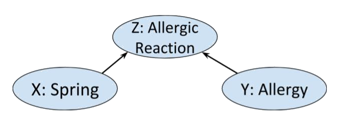
Clearly whether or not Alice has allergies other than hayfever is independent of what season it is. So we’d expect a distribution on this graph to satisfy $X \perp\!\!\!\!\!\!\!\perp Y \ | \ \emptyset$. However, if we know that Alice is having an allergic reaction, and it happens to be spring, we will likely assume that she has some allergy, i.e. $X$ and $Y$ are not conditionally independent given $Z$.

Indeed, the Markov condition and chain rule for this graph gives us $X \perp\!\!\!\!\!\!\!\perp Y \ | \ \emptyset$:

$$P(x, y, z) = P(x)P(y) P(z \ | \ x,\ y) = P(z \ | \ x,\ y) P( x\ | \ y) P(y) \ \forall x,y,z.$$

from which we cannot derive $P(x \ | \ z) P(y \ | \ z) = P(x,y \ | \ z)$. (However, it could still be true for some particular choice of probability distribution.)

Chain

Finally, let us return to the chain of correlations presented in the introduction.

Clearly the probabilities that it is spring and that Alice is sneezing are not independent, and indeed, we cannot derive $P(x, y) = P(x) P(y)$. However observe that, by the chain rule, a Markov distribution on the chain graph must satisfy $X\perp\!\!\!\!\!\!\!\perp Y \ | \ Z$. If we know Alice is having an allergic reaction that is not hayfever, whether or not she is sneezing is not going to affect our guess as to what season it is.

Crucially, in this case, knowing the season is also not going to affect whether we think Alice is sneezing. By definition, conditional independence of $X$ and $Y$ given $Z$ is symmetric in $X$ and $Y$. In other words, a joint distribution $P$ on the variables $X,Y,Z$ satisfies the Markov condition with respect to the chain graph

$$X \longrightarrow Z \longrightarrow Y$$

if and only if $P$ satisfies the Markov condition on

$$Y \longrightarrow Z \longrightarrow X .$$

d-separation

The above observations can be generalised to statements about conditional independences in any Bayesian network. That is, if $(G,P)$ is a Bayesian network then the structure of $G$ is enough to derive all the conditional independences in $P$ that are implied by the graph $G$ (in reality there may be more that have not been included in the network!).

Given a DAG $G$ and a set of vertices $U$ of $G$, let $m(U)$ denote the union of $U$ with all the vertices $v$ of $G$ such that there is a directed edge from $U$ to $v$. The set $W(U)$ will denote the non-inclusive future of $U$, that is, the set of vertices $v$ of $G$ for which there is no directed (possibly trivial) path from $v$ to $U$.

For a graph $G$, let $X, Y, Z$ now denote disjoint subsets of the vertices of $G$ (and their corresponding random variables). Set $W := W(X \cup Y \cup Z)$.

Then $X$ and $Y$ are said to be d-separated by $Z$, written $X \perp Y \ | \ Z$, if there is a partition $\{U,V,W,Z\}$ of the nodes of $G$ such that

• $X \subseteq U$ and $Y \subseteq V$, and

• $m(U) \cap m(V) \subseteq W,$ in other words $U$ and $V$ have no direct influence on each other.

(This is lemma 19 in the paper.)

Now d-separation is really useful since it tells us everything there is to know about the conditional dependences on Bayesian networks with underlying graph $G$. Indeed,

Theorem 5

• Soundness of d-separation (Verma and Pearl, 1988) If $P$ is a Markov distribution with respect to a graph $G$ then for all disjoint subsets $X,Y,Z$ of nodes of $G$ $X \perp Y \ | \ Z$ implies that $X \perp\!\!\!\!\!\!\!\perp Y \ | \ Z$.

• Completeness of d-separation (Meek, 1995) If $X \perp\!\!\!\!\!\!\!\perp Y \ | \ Z$ for all $P$ Markov with respect to $G$, then $X \perp Y \ | \ Z$.

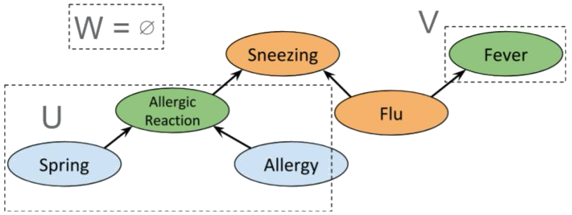
We can combine the previous examples of fork, collider and chain graphs to get the following

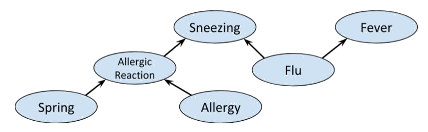
A priori, Allergic reaction is conditionally independent of Fever. Indeed, we have the partition

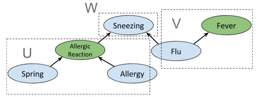
which clearly satisfies d-separation. However, if Sneezing is known then $W = \emptyset$, so Allergic reaction and Fever are not independent. Indeed, if we use the same sets $U$ and $V$ as before, then $m(U) \cap m(V) = \{ Sneezing \}$, so the condition for d-separation fails; and it does for any possible choice of $U$ and $V$. Interestingly, if Flu is also known, we again obtain conditional independence between Allergic reaction and Fever, as shown below.

Before describing the limitations of this setup and why we may want to generalise it, it is worth observing that Theorem 5 is genuinely useful computationally. Theorem 5 says that given a Bayesian network $(G,P)$, the structure of $G$ gives us a recipe to factor $P$, thereby greatly increasing computation efficiency for Bayesian inference.

Latent variables, hidden variables, and unobservables

In the context of Bayesian networks, there are two reasons that we may wish to add variables to a probabilistic model, even if we are not entirely sure what the variables signify or how they are distributed. The first reason is statistical and the second is physical.

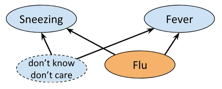
Consider the example of flu, fever and sneezing discussed earlier. Although our analysis told us $Fever \perp\!\!\!\!\!\!\!\perp Sneezing \ | \ Flu$, if we conduct an experiment we are likely to find:

$$P(fever \ | \ sneezing, \ flu) \neq P(fever \ | \ flu).$$

The problem is caused by the graph not properly modelling reality, but a simplification of it. After all, there are a whole bunch of things that can cause sneezing and flu. We just don’t know what they all are or how to measure them. So, to make the network work, we may add a hypothetical latent variable that bunches together all the unknown joint causes, and equip it with a distribution that makes the whole network Bayesian, so that we are still able to perform inference methods like belief propagation.

On the other hand, we may want to add variables to a Bayesian network if we have evidence that doing so will provide a better model of reality.

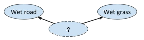
For example, consider the network with just two connected nodes

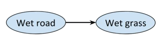
Every distribution on this graph is Markov, and we would expect there to be a correlation between a road being wet and the grass next to it being wet as well, but most people would claim that there’s something missing from the picture. After all, rain could be a ‘common cause’ of the road and the grass being wet. So, it makes sense to add a third variable.

But maybe we can’t observe whether it has rained or not, only whether the grass and/or road are wet. Nonetheless, the correlation we observe suggests that they have a common cause. To deal with such cases, we could make the third variable hidden. We may not know what information is included in a hidden variable, nor its probability distribution.

All that matters is that the hidden variable helps to explain the observed correlations.

So, latent variables are a statistical tool that ensure the Markov condition holds. Hence they are inherently classical, and can, in theory, be known. But the universe is not classical, so, even if we lump whatever we want into as many classical hidden variables as we want and put them wherever we need, in some cases, there will still be empirically observed correlations that do not satisfy the Markov condition.

Most famously, Bell’s experiment shows that it is possible to have distinct variables $A$ and $B$ that exhibit correlations that cannot be explained by any classical hidden variable, since classical variables are restricted by the principle of locality.

In other words, though $A \perp B \ | \ \Lambda$,

$$P(a \ | b,\ \lambda) \neq P(a \ | \ \lambda).$$

Implicitly, this means that a classical $\Lambda$ is not enough. If we want $P(a \ | b,\ \lambda) \neq P(a \ | \ \lambda)$ to hold, $\Lambda$ must be a non-local (non-classical) variable. Quantum mechanics implies that we can’t possibly empirically find the value of a non-local variable (for similar reasons to the Heisenberg’s uncertainty principle), so non-classical variables are often called unobservables. In particular, it is irrelevant to question whether $A \perp\!\!\!\!\!\!\!\perp B \ | \ \Lambda$, as we would need to know the value of $\Lambda$ in order to condition over it.

Indeed, this is the key idea behind what follows. We declare certain variables to be unobservable and then insist that conditional (in)dependence only makes sense between observable variables conditioned over observable variables.

Generalising classical causality

The correlations observed in the Bell experiment can be explained by quantum mechanics. But thought experiments such as the one described here suggest that theoretically, correlations may exist that violate even quantum causality.

So, given that graphical models and d-separation provide such a powerful tool for causal reasoning in the classical context, how can we generalise the Markov condition and Theorem 5 to quantum, and even more general causal theories? And, if we have a theory-independent Markov condition, are there d-separation results that don’t correspond to any given causal theory?

Clearly the first step in answering these questions is to fix a definition of a causal theory.

Operational probabilistic theories

An operational theory is a symmetric monoidal category $(\mathsf {C}, \otimes, I)$ whose objects are known as systems or resources. Morphisms are finite sets $f = \{\mathcal {C}_i\}_{i \in I}$ called tests, whose elements are called outcomes. Tests with a single element are called deterministic, and for each system $A \in ob (\mathsf {C})$, the identity $id_A \in \mathsf (A,A)$ is a deterministic test.

In this discussion, we’ll identify tests $\{\mathcal {C}_i \}_i , \{\mathcal {D}_j\}_j$ in $\mathsf {C}$ if we may always replace one with the other without affecting the distributions in $\mathsf {C}(I, I)$.

Given $\{\mathcal {C}_i \}_i \in \mathsf {C}(B, C)$ and $\{\mathcal {D}_j \} \in \mathsf {C}(A, B)$, their composition $f \circ g$ is given by

$$\{ \mathcal {C}_i \circ \mathcal {D}_j \}_{i,j} \in \mathsf {C}(A, C).$$

First apply $\mathcal {D}$ with output $B$ then apply $\mathcal {C}$ with outcome $C$.

The monoidal composition $\{ \mathcal {C}_i \otimes \mathcal {D}_j \}_{i, j} \in \mathsf {C}(A \otimes C, B \otimes D)$ corresponds to applying $\{\mathcal {C}_i\}_i \in \mathsf {C}(A,B)$ and $\{ \mathcal {D}_j \}_j$ separately on $A$ and $C$.

An operational probabilistic theory or OPT is an operational theory such that every test $I \to I$ is a probability distribution.

A morphism $\{ \mathcal {C}_i \}_i \in \mathsf {C}(A, I)$ is called an effect on $A$. An OPT $\mathsf {C}$ is called causal or a causal theory if, for each system $A \in ob (\mathsf {C})$, there is a unique deterministic effect $\top_A \in \mathsf {C}( A, I)$ which we call the discard of $A$.

In particular, for a causal OPT $\mathsf {C}$, uniqueness of the discard implies that, for all systems $A, B \in ob (\mathsf {C})$,

$$\top_A \otimes \top_B = \top_{A \otimes B},$$ and, given any determinstic test $\mathcal {C} \in \mathsf {C}(A, B)$,

$$\top_B \circ \mathcal {C} = \top_A.$$

The existence of a discard map allows a definition of causal morphisms in a causal theory. For example, as we saw in January when we discussed Kissinger and Uijlen’s paper, a test $\{ \mathcal {C}_i \}_i \in \mathsf {C} (A, B)$ is causal if

$$\top_B \circ \{ \mathcal {C}_i \}_i = \top_A \in \mathsf {C}( A, I).$$

In other words, for a causal test, discarding the outcome is the same as not performing the test. Intuitively it is not obvious why such morphisms should be called causal. But this definition enables the formulation of a non-signalling condition that describes the conditions under which the possibility of cause-effect correlation is excluded, in particular, it implies the impossibility of time travel.

Examples

The category $Mat(\mathbb {R}_+)$ of natural numbers and with $Mat(\mathbb {R}_+)(m,n)$ the set of $n \times m$ matrices, has the structure of a causal OPT. The causal morphisms in $Mat(\mathbb {R}_+)$ are the stochastic maps (the matrices whose columns sum to 1). This category describes classical probability theory.

The category $\mathsf{CPM}$ of sets of linear operators on Hilbert spaces and completely positive maps between them is an OPT and describes quantum relations. The causal morphisms are the trace preserving completely positive maps.

Finally, Boxworld is the theory that allows to describe any correlation between two variables as the cause of some resource of the theory in the past.

Generalised Bayesian networks

So, we’re finally ready to give the main construction and results of the paper. As mentioned before, to get a generalised d-separation result, the idea is that we will distinguish observable and unobservable variables, and simply insist that conditional independence is only defined relative to observable variables.

To this end, a generalised DAG or GDAG is a DAG $G$ together with a partition on the nodes of $G$ into two subsets called observed and unobserved. We’ll represent observed nodes by triangles, and unobserved nodes by circles. An edge out of an (un)observed node will be called (un)observed and represented by a (solid) dashed arrow.

In order to get a generalisation of Theorem 5, we still need to come up with a sensible generalisation of the Markov property which will essentially say that at an observed node that has only observed parents, the distribution must be Markov. However, if an observed node has an unobserved parent, the latter’s whole history is needed to describe the distribution.

To state this precisely, we will associate a causal theory $(\mathsf {C}, \otimes, I)$ to a GDAG $G$ via an assignment of systems to edges of $G$ and tests to nodes of $G$, such that the observed edges of $G$ will ‘carry’ only the outcomes of classical tests (so will say something about conditional probability) whereas unobserved edges will carry only the output system.

Precisely, such an assignment $P$ satisfies the generalised Markov condition (GMC) and is called a generalised Markov distribution if

• Each unobserved edge corresponds to a distinct system in the theory.

• If we can’t observe what is happening at a node, we can’t condition over it: To each unobserved node and each value of its observed parents, we assign a deterministic test from the system defined by the product of its incoming (unobserved) edges to the system defined by the product of its outgoing (unobserved) edges.

• Each observed node $X$ is an observation test, i.e. a morphism in $\mathsf {C}(A, I)$ for the system $A \in ob( \mathsf {C})$ corresponding to the product of the systems assigned to the unobserved input edges of $X$. Since $\mathsf {C}$ is a causal theory, this says that $X$ is assigned a classical random variable, also denoted $X$, and that if $Y$ is an observed node, and has observed parent $X$, the distribution at $Y$ is conditionally dependent on the distribution at $X$ (see here for details).

• It therefore follows that each observed edge is assigned the trivial system $I$.

• The joint probability distribution on the observed nodes of $G$ is given by the morphism $\mathsf {C}(I, I)$ that results from these assignments.

A generalised Bayesian network consists of a GDAG $G$ together with a generalised Markov distribution $P$ on $G$.

Example

Consider the following GDAG

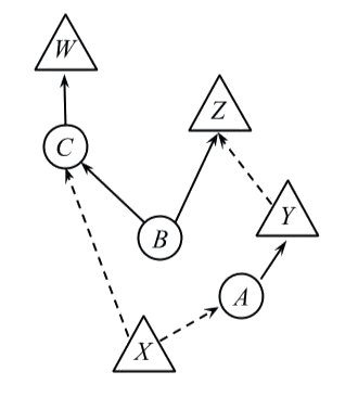
Let’s build its OPT morphism as indictated by the generalised Markov condition.

The observed node $X$ has no incoming edges so it corresponds to a $\mathsf {C}(I, I)$ morphism, and thus we assign a probability distribution to it.

The unobserved node A depends on $X$, and has no unobserved inputs, so we assign a deterministic test $A(x): I \to A$ for each value $x$ of $X$.

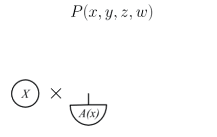
The observed node $Y$ has one incoming unobserved edge and no incoming observed edges so we assign to it a test $Y: A \to I$ such that, for each value $x$ of $X$, $Y \circ A(x)$ is a probability distribution.

Building up the rest of the picture gives an OPT diagram of the form

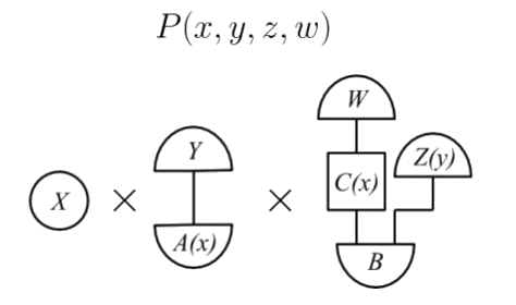
which is a $\mathsf {C}(I, I)$ morphism that defines the joint probability distribution $P(x,y,z,w)$. We now have all the ingredients to state Theorem 22, the generalised d-separation theorem. This is the analogue of Theorem 5 for generalised Markov distributions.

Theorem 22

Given a GDAG $G$ and subsets $X,Y, Z$ of observed nodes

• if a probability distribution $P$ is generalised Markov relative to $G$ then $X \perp Y \ | \ Z \Rightarrow X\perp\!\!\!\!\!\!\!\perp Y \ | \ Z$.

• If $X\perp\!\!\!\!\!\!\!\perp Y \ | \ Z$ holds for all generalised Markov probability distributions on $G$, then $X \perp Y \ | \ Z$.

Note in particular that there is no change in the definition of d-separation: d-separation of a GDAG $G$ is simply d-separation with respect to its underlying DAG. There is also no change in the definition of conditional independence. Now, however, we restrict to statements of conditional independence with respect to observed nodes only. This enables the generalised soundness and completeness statements of the theorem.

The proof of soundness uses uniqueness of discarding, and completeness follows since generalised Markov is a stronger condition on a distribution than classically Markov.

Classical distributions on GDAGs

Theorem 22 is all well and good. But does it really generalise the classical case? That is, can we recover Theorem 5 for all classical Bayesian networks from Theorem 22?

As a first step, Proposition 17 states that if all the nodes of a generalised Bayesian network are observed, then it is a classical bayesian network. In fact, this follows pretty immediately from the definitions.

Moreover, it is easily checked that, given a classical Bayesian network, even if it has hidden or latent variables, it can still be expressed directly as a generalised Bayesian network with no unobserved nodes.

In fact, Theorem 22 generalises Theorem 5 in a stricter sense. That is, the generalised Bayesian network setup together with classical causality adds nothing extra to the theory of classical Bayesian networks. If a generalised Markov distribution is classical (then hidden and latent variables may be represented by unobserved nodes), it can be viewed as a classical Bayesian network. More precisely, Lemma 18 says that, given any generalised Bayesian network $(G,P)$ with underlying DAG $G'$ and distribution $P \in \mathcal {C}$, we can construct a classical Bayesian network $(G', P')$ such that $P'$ agrees with $P$ on the observed nodes.

It is worth voicing a note of caution. The authors themselves mention in the conclusion that the construction based on GDAGs with two types of nodes is not entirely satisfactory. The problem is that, although the setups and results presented here do give a generalisation of Theorem 5, they do not, as such, provide a way of generalising Bayesian networks as they are used for probabilistic inference to non-classical settings. For example, belief propagation works through observed nodes, but there is no apparent way of generalising it for unobserved nodes.

Theory independence

More generally, given a GDAG $G$, we can look at the set of distributions on $G$ that are generalised Markov with respect to a given causal theory. Of particular importance are the following.

• The set $\mathcal {C}$ of generalised Markov distributions in $Mat(\mathbb {R}_+)$ on $G$.

• The set $\mathcal {Q}$ of generalised Markov distributions in $\mathsf{CPM}$ on $G$.

• The set $\mathcal {G}$ of all generalised Markov distributions on $G$. (This is the set of generalised Markov distributions in Boxworld.)

Moreover, we can distinguish another class of distributions on $G$, by not restricting to d-seperation of observed nodes, but considering distributions that satisfy the observable conditional independences given by any d-separation properties on the graph. Theorem 22 implies, in particular that $G \subseteq I$.

And, so, since $Mat(\mathbb {R}_+)$ embeds into $\mathsf{CPM}$, we have $\mathcal {C} \subseteq \mathcal {Q} \subseteq \mathcal {G} \subseteq \mathcal {I}$.

This means that one can ask for which graphs (some or all of) these inequalities are strict, and the last part of the paper explores these questions. In the original paper, a sufficient condition is given for graphs to satisfy $\mathcal {C} \neq \mathcal {I}$. I.e. for these graphs it is guaranteed that the causal structure admits correlations that are non-local. Moreover the authors show that their condition is necessary for small enough graphs.

Another interesting result is that there exist graphs for which $\mathcal {G} \neq \mathcal {I}$. This means that using a theory of resources, whatever theory it may be, to explain correlations imposes constraints that are stronger than those imposed by the relations themselves.

What next?

This setup represents one direction for using category theory to generalise Bayesian networks. In our group work at the ACT workshop, we considered another generalisation of Bayesian networks, this time staying within the classical realm. Namely, building on the work of Bonchi, Gadducci, Kissinger, Sobocinski, and Zanasi, we gave a functorial Markov condition on directed graphs admitting cycles. Hopefully we’ll present this work here soon.